Evaluating Model Uncertainty

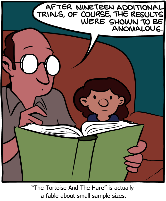
A study with n=1 has large uncertainty. Source: SMBC.

Overview

Quantifying uncertainty is an important part of model evaluation. During model building and selection, we are not only interested in some point estimate of model performance (e.g., average RMSE), but would often also like to know how that performance measure is distributed and how it differs between models. For instance, we might have 2 classification models, one with an average accuracy (obtained through CV) of 70%, while the other has 80%. It looks like we should go with model 2, right? But what if we also knew that the range of accuracy values (for different repeats of the CV) is 65% - 75% for model 1, and it is 45% - 95% for model 2. Which model do we prefer? We might still prefer model 2, but there is also an argument that we might want to go with model 1, which has better performance at the lower bound. Without knowing the distribution of performance measures, we can only make limited decisions.

For our “final” model, we are most often interested in the uncertainty associated with predictions of outcomes. At times, we might also be interested in the values of model parameters and thus might want to know uncertainty associated with those estimates.

Model performance uncertainty

If we perform cross-validation, (often repeated), we get multiple estimates for model performance based on the test set performance. For instance, in 10-fold CV 10 times repeated, we get 100 values for the model performance metric (e.g., RMSE). We can look at the distribution of those RMSE. While the standard approach is to pick a model with lower mean RMSE (or other performance measures), that doesn’t have to be the case. We might prefer one with a somewhat higher mean but less variance, as in the example above. Or we could pick a model with a “small enough” RMSE that makes the model less complex, e.g. including less predictors (what “small enough” means has to be defined by you). To that end, looking at distributions of model performance is useful.

Model parameter uncertainty

At times, we might be interested in knowing the uncertainty of the model parameters. This will also give us the uncertainty in the predicted expected values of the model. Both of those quantities, uncertainty in parameters and model expectations can be quantified with confidence intervals. (Or the Bayesian equivalent of credible intervals).

Some functions in R, e.g. lm() have a built-in command to compute confidence intervals. For more complex models or approaches, such built-in functions might not exist. A general approach to produce confidence or prediction intervals is with a sampling method that is very similar in spirit to cross-validation, namely by performing bootstrapping.

Bootstrapping

The idea for bootstrapping is fairly straightforward. Bootstrapping tries to imitate a scenario in which you repeated your study and collected new data. Instead of having actual new data, the idea is that the existing data is sampled to form a new “dataset”, which is then fit. Sampling is performed with replacement to obtain a sample the size of the original dataset. Some observations now show up more than once, and some do not show up. For each such sample, you fit your model and estimate parameters. You will thus get a distribution of parameter estimates. From those distributions, you can compute confidence intervals, e.g., the usual 95% interval. For each fit, you can also predict outcomes and thus obtain a distribution of prediction outcomes (see next).

Like cross-validation, the bootstrap method is very general and can be applied to pretty much any problem. If your data has a specific structure, you can adjust the sampling approach (e.g., if you have observations from different locations, you might want to sample with replacement for each location.) Limitations for the bootstrap are that you need a decent amount of data for it to work well, and since you are repeating this sampling procedure many times, the procedure can take a while to run.

Model prediction uncertainty

If we are interested in model predictions, we generally also want to know how much uncertainty is associated with those predictions. For continuous outcomes, computing prediction intervals gives an idea of the uncertainty in our predictions. As for parameter uncertainty, some R functions have built-in methods to compute prediction intervals, or you can use the bootstrap approach.

Note that prediction intervals are not the same as confidence intervals. The latter quantifies the uncertainty in model parameters, e.g., the b_i in a regression model. Since those b_i have uncertainty, the model predictions for the expected observation has uncertainty. However, each real observation has additional scatter around the expected value. This additional uncertainty needs to be factored in when trying to make predictions for individual outcomes. As such, prediction intervals are wider than confidence intervals.

P-values

So what about the p-value? This quantity doesn’t measure uncertainty directly, though it is in some way related to it. p-values are sometimes useful for hypothesis testing. But in my opinion, p-values are overused, generally not too meaningful, and can most often be skipped (though sometimes one needs them just to make reviewers happy). I’m thus not talking about them further.

Further learning

Bootstrapping is discussed in the Resampling Methods chapter of ISLR and the Cross Validation chapter of IDS. The other topics are covered in various places in the different course materials we’ve been using, but again not in any full chapters/sections. So if you have suggestions for good resources, let me know.