Chapter 5 Reproductive Number

5.1 Overview and Learning Objectives

The reproductive number is a fundamental concept in infectious disease epidemiology. It is so important, it even made its way into (at least) one mainstream movie (“Contagion” 2011)! It is simple in its definition and rather useful. The hard part is to correctly estimate the reproductive number for a given disease and scenario. We will discuss all these aspects in the following.

The learning objectives for this chapter are:

• Know how the reproductive number is defined
• Kow how to compute the reproductive number from data
• Apply the reproductive number concept to ID control

5.2 Introduction

We generally want to prevent infectious diseases from causing outbreaks, stop already ongoing outbreaks, reduce the number of people getting infected, or even bolder, try to eradicate a disease. If we were able to make a vaccine against an infectious disease, it is useful to know what fraction of the population should be vaccinated to prevent future outbreaks or even eradicate the disease.

Assume you asked the “person on the street” the question: “If we wanted to prevent a potential future SARS outbreak, what fraction of the U.S. population do we need to vaccinate to make a large-scale outbreak impossible?” I suspect that most people would likely say that nearly everyone needs to be vaccinated to prevent outbreaks. A smaller number of people might realize that we don’t need to vaccinate everyone, just enough people to sufficiently reduce the disease’s transmission potential. To reach the second answer, one needs to have thought about how infectious diseases ‘work.’

If you happen to come across an ID public health specialist or ID modeler, you might get a different answer. Namely, they might provide you with a quantitative estimate of the fraction of people that need to get vaccinated. They might, for instance, tell you that we would need to vaccinate around 70% of the population. This is, of course, the best kind of information. How do we figure this out? That’s where the reproductive number concept comes into play.

5.3 Reproductive number definition

The concept and definition of the reproductive number are rather straightforward: The reproductive number (usually abbreviated with R), is defined as the average number of secondary infectious cases caused by one infectious individual (before they recover or die or are otherwise not able to further transmit). The following figure illustrates the concept.

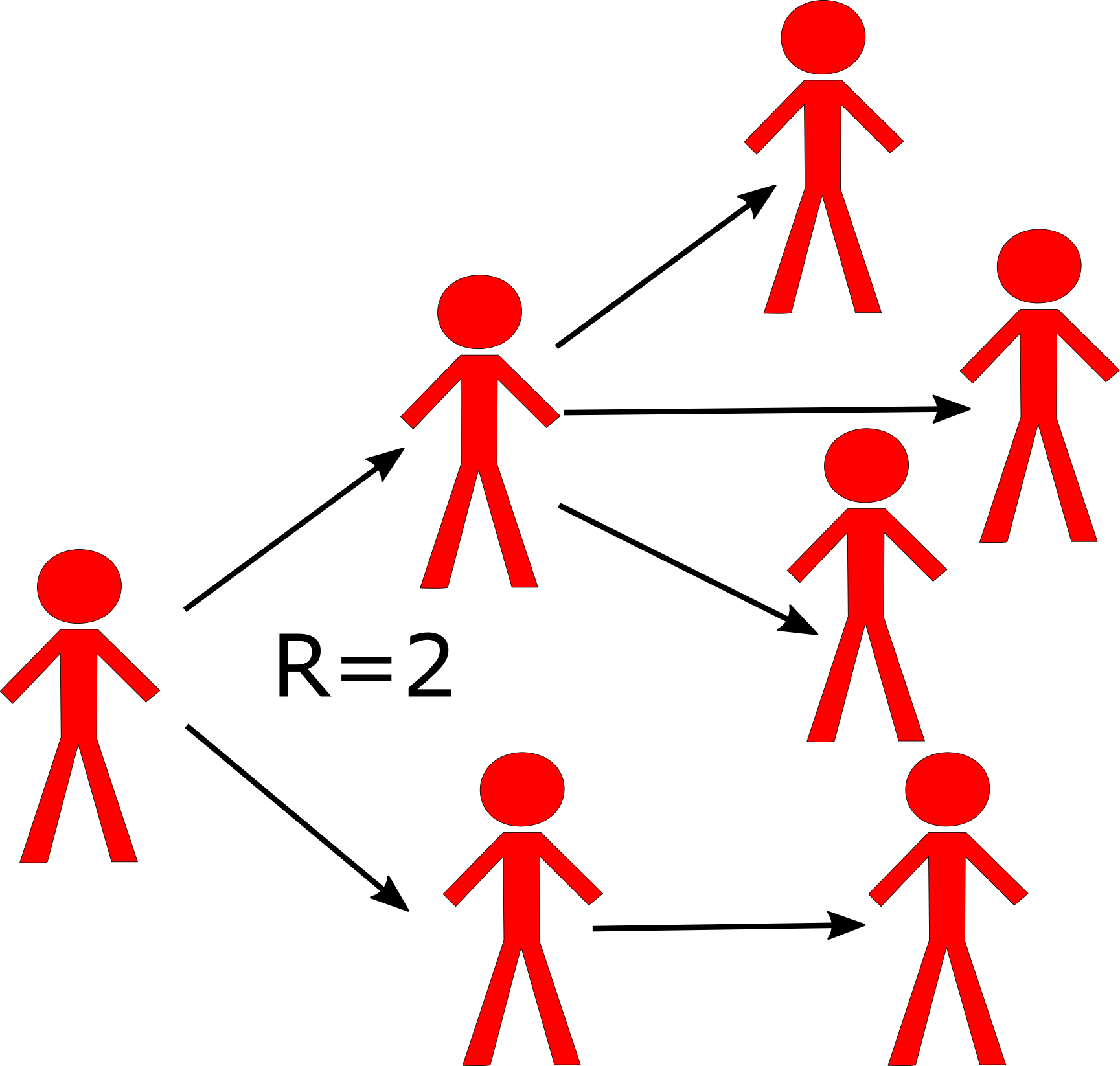
Schematic showing the definition of the reproductive number. Each person `produces’ on average 2 other infectious individuals. (Of course, we would usually need to have more data than shown in this figure to properly estimate R.)

From this definition of the reproductive number, it is clear that if the value is greater than 1, the pathogen keeps spreading to more and more people and we have a growing outbreak. Conversely, if R is less than 1, the outbreak will fizzle out. Because of this characteristic, it is important to know R for a given outbreak, which will then tell us how stringent the interventions need to be to bring the outbreak under control. This is more explained in the following sections.

5.4 Reproductive number details

Let’s look a bit closer at the definition for R. First, note that it applies to population averages. A single person might infect none, a few or many others. R does not capture this detail. It only describes the average. That’s why it is, for instance, possible to have R=2.5 or other non-integer numbers. Of course, it is not possible for an individual to infect 2.5 others, but since R describes an average, such fractional infections are possible. This population average feature of R is a strength since it makes R relatively easy to determine. It is also a weakness since often we’d like to know the distribution in addition to the mean/average - we’ll discuss that when we deal with ideas such as population heterogeneity, core groups, and super-spreaders in later chapters.

Another point to note is that the definition is about the number of new infectious hosts produced by one infectious host. For some diseases, being infected and being infectious are pretty much the same. E.g. pretty much everyone who is infected with HIV is also - to some degree - infectious. For other diseases, that is not the case. For instance, the majority of people who get infected with TB will never reach a state where they are infectious. To compute R, we do not count the average number of individuals an infectious person infects, but only those that later go on to become infectious themselves. The same idea applies when we talk about diseases that have multiple hosts. R is defined as the number of infectious hosts ‘produced’ by one infectious host of the same type. For instance, for vector-borne diseases, R would be the number of infectious humans ‘produced’ by one infectious human via the intermediary mosquito/vector stage. While conceptually still straightforward, measuring and computing R/R₀ in such multi-host situations can get tricky.

5.5 Basic reproductive number

A special case of the reproductive number is at the beginning of an outbreak when essentially everyone in the population is susceptible. In this case, when we assume everyone is susceptible, we define a special quantity called the basic reproductive number, abbreviated as R₀. The quantity R₀ is a measurement of the transmission potential of a disease in a particular setting. It does by definition not change during an ongoing outbreak. The more general definition of the reproductive number, R, does change during an epidemic. We’ll discuss that more below.

5.6 Reproductive number terminology

While I will be mainly using the term reproductive number, there are alternative names for R. In general, any combination of reproductive/reproduction and ratio/number is ok terminology. In its early days, R was called reproductive rate. This is incorrect terminology and should not be used. R is not a rate (there are no units of inverse time). Why does that matter? See the ‘R is not a rate’ box for an example. Unfortunately, old habits die slowly and you can still see the word `rate’ applied to the reproductive number in some recent publications.

5.6.0.1 Why R Is Not a Rate - Example

It is important to understand that R only provides a measure of how transmissible a pathogen is, R does not provide any information about the speed at which transmission occurs. This is an important limitation of R. Consider 2 infections with the similar reproductive number, say HIV and SARS, which are both estimated to have a reproductive number of around 3-4. If we let an outbreak ‘run its course,’ we would - based on R - expect to get the same number of infected individuals. However, the dynamics at which those infections occur will be quite different. SARS spreads rapidly, i.e. an infected person infects 3-4 others within a few weeks. On the other hand, a person infected with HIV will infect others on a timeframe of years. These different dynamics have of course important implications on the control approaches against diseases. Thus, while knowing R is significant for a given disease, it doesn’t tell ‘the full story.’

5.6.0.2 Notes

While we often say “Infectious disease X has an R₀ of Y,” this is only an approximation. R and R₀ also depend on the setting. The potential for transmission for many ID is much higher in for instance crowded locations (prisons, slums, cruise ships), or among “high risk groups” (e.g. STD in sex workers). For example in most countries R₀ of HIV is below 1 in the general population but HIV is not disappearing because it has an R₀ > 1 in certain subgroups. The importance of such population heterogeneity is further discused in chapter 10 . When we talk about R, it is therefore useful to be as specific as possible about the scenario/population/setting.

In this book, and in the literature in general, you will often find the use of R₀, R or effective R (R_eff) used (sloppily) in an interchangeable manner. Usually, it is clear from the context if the symbol refers specifically to R₀ at the beginning of an outbreak in a susceptible population, or more generally to R, the average number of secondary infectious cases produced by one infectious individual in any population.

Unfortunately, R seem to be a very popular letter. In the context of infectious disease dynamics, R is used both to indicate the removed compartment in an SIR model, and as abbreviation for the reproductive number. To make things worse, it is also the name of the programming language which I used to write the DSAIDE package which accompanies this book. You will just have to figure out from the context if a reference to R means “computer software” or “removed compartment” or “reproductive number.” Fortunately, it should always be clear what is meant.

5.7 Outbreaks and the Change in R

As stated above, at the beginning of an outbreak, a specific disease in a certain setting will have some value R₀. As the outbreak progresses, more and more hosts become infected and - for many diseases - either die or recover and become immune to further infection. This leads to a reduction in the reproductive number as the outbreak progresses. For instance, at the start of the epidemic with everyone susceptible, R₀=3. Then once a third of the population have become infected and immune, an infectious person who would have infected three others at the beginning of an outbreak now ‘wastes’ one of their transmissions on an already immune person, and therefore only infects two others. Similarly, once 2/3 of the population have become infected and immune, R will have dropped to 1. The outbreak has reached its peak. From our definition, when R=1, the outbreak does not grow further nor does it decay (recall, we need R>1 for growth or R<1 for decay). However, this point of the outbreak, the peak with R=1, is somewhat instantaneous as, now, more than 2/3 of the population have become infected or immune which causes R to drop below 1. Thus, the outbreak starts to decline, with R continuing to go down as fewer and fewer susceptibles remain.

5.8 Reproductive Number and Outbreak Control

It is intuitively clear that if on average every infectious person “produces” more than one subsequent infectious person, we get a growing epidemic. In contrast, if every infectious person “produces” less than one subsequent infectious person, the pathogen might transmit a few times, but pretty soon it will disappear. Thus if we can achieve R < 1, e.g. through vaccination, we can prevent an outbreak from starting. Further, if during an outbreak we can intervene to get R < 1, the outbreak is going to fizzle out. Figure 5.1 illustrates this idea. If we wanted to stop any further transmission, we would need to get R even lower, namely R = 0. Intervention efforts try to achieve an R as small as possible. If we could achieve R < 1 globally everywhere, we could eventually eradicate a disease. The ability to do that depends on many factors. One important one is the R₀ value of any ID before we start an eradication campaign. Intuitively, the higher R₀, the harder it will be to get it to < 1. We’ll make that more explicit below.

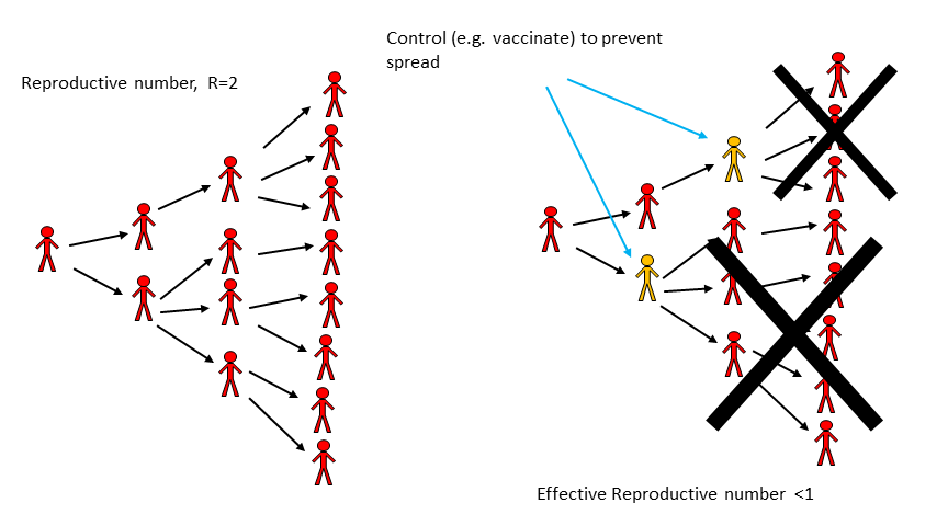
FIGURE 5.1: Impact of an Intervention on transmission.

5.8.0.1 R and Outbreak Control - Example

During the large Ebola outbreak in West Africa which started in 2013, a few Ebola patients came to the U.S., and the goal was to have R = 0, i.e. no ongoing transmission. That didn’t quite happen, a few new individuals got infected, but R was very close to zero. In contrast, in West Africa, there was little hope to get R = 0 quickly. Fortunately, R < 1 is enough. So we can ‘tolerate’ a few further transmissions and new cases and still get the outbreak under control eventually. Of course, in general, we want to get R as close to 0 as possible, especially for a disease as deadly as Ebola. But to get an outbreak to fizzle out, we only need R < 1, not R = 0.

5.9 Estimating Intervention Efforts based on R

Let’s make the relation between response efforts and the reproductive number a bit more quantitative. As a simple example, consider an infectious disease with R₀=2. That means on average every infected person infects two others. If we could somehow protect a bit more than half of the susceptibles, then a person who might have become infected can’t become infected anymore, and the effective R (sometimes called R_eff) drops below 1. More generally, to prevent an outbreak, a fraction p = 1-1/R₀ of the population needs to be protected (e.g. through vaccination). From this, it follows that the higher R₀, the harder it is to control and ID. This is illustrated in figure 5.2. One can see both from the figure and the equation that a disease with say R₀ = 5 requires that 80% of the population is protected such that R_eff = 1.

The level of population protection at which R=1 is called critical population (or herd) immunity level. The relation between basic reproductive number, intervention coverage, and effective R is R= R₀(1-p). That holds true if we assume that the intervention fully protects those to whom it is applied. If the intervention is not perfect, we have R=R₀(1-e*p), where _e is the effectiveness of the intervention (_e=1 is an entirely effective intervention).

FIGURE 5.2: R₀ and Interventions. From (Matt J. Keeling and Rohani 2008).

5.9.0.1 Rearranging the Herd Immunity Equation

If we take our equation \(R=R_0(1-p)\) and substitute \(R=1\) then solve for _p, we get \(P_{HI}=1-\frac{1}{R_0}\), or if we include vaccine efficacy, we get the equation as below.

\[ \begin{aligned} R = R_0(1-e*p) \\ 1 = R_0(1-e*p) \\ \frac{1}{R_0} = 1-e*p \\ e*p = 1 - \frac{1}{R_0} \\ p = (1-\frac{1}{R_0})(\frac{1}{e}) \\ \end{aligned} \]

Measles has an R_0 of ~15. Let’s plug this value into our new equation for the critical population immunity level, i.e., the proportion of the population who need to be immune to establish herd immunity.

\[ \begin{aligned} p = (1 - \frac{1}{R_0})(\frac{1}{e}) \\ p = (1 - \frac{1}{15})(\frac{1}{e}) \\ p \approx 0.933 \times (\frac{1}{e}) \\ \end{aligned} \]

So, what does this mean? For a perfectly efficacious vaccine, i.e., \(e=1\), we would need 93.3% to be immune to measles to prevent outbreaks. We can reach this 93.3% by natural immunity (i.e., developing immunity following infection) or by inducing artificial immunity (e.g., actively via vaccination). The Measles, Mumps, Rubella (MMR) vaccine is our currently best option for inducing artificial immunity. CDC states that one dose of MMR is 93% effective against measles and that two doses are 97% effective (Immunization and Diseases 2019). How do these numbers affect our calculations of critical population immunity level. Well, for one dose \(p \approx 0.933 \times \frac{1}{0.93} \approx 1.003\). This is an illogical value as it indicates that over 100% of the population would need to be vaccinated to reach herd immunity. Why? Because the vaccine effectiveness is less than the critical population immunity level; that is, even if 100% of people were vaccinated only 93% of them would become immune and, thus, there would still be enough susceptibles to allow an outbreak to happen. For two doses, \(p \approx 0.933 \times \frac{1}{0.97} \approx 0.962\). This means that 96.2% of a population would need to be vaccinated (i.e., given two doses of MMR) to prevent an outbreak of measles. Perhaps with this knowledge, you can understand how vaccination hesitancy and refusal debates often mention measles.

5.9.0.2 R and the SIR Model

We can connect the concept that R>1 leads to growth and R<1 leads to a decline in infectious persons with the simple SIR model for an outbreak. The model, which we saw earlier, is given by the following set of differential equations (Don’t confuse the R for the recovered with the R/R₀ from the reproductive number. Unfortunately it is customary to use the same letter for both.):

\[ \begin{aligned} \dot S &= - b SI \\ \dot I &= b S I - g I \\ \dot R &= g I \end{aligned} \] For this model, what needs to be true to get an increase in the number of infectious hosts? The influx of new infectious hosts, bSI, needs to be larger than the outflow, gI. This condition, bSI > gI, can be rewritten as 1 < (bS)/g. We then define the quantity on the right side of this condition as the reproductive number, R = (bS)/g. At the beginning of an outbreak, where everyone is assumed to be susceptible (written as S= S₀), we have the special case of the basic reproductive number, R₀ = (bS₀)/g. Note that the rate of recovery, g, is related to the average duration of infection, D as D=1/g. Therefore, one can also write R = DbS, with the special case R₀ for S=S₀, i.e. at the beginning of an outbreak.

5.10 How to determine R

Knowing the reproductive number for a particular pathogen and scenario is important to allow for adequate intervention planning. There are multiple ways to estimate R from data. We’ll briefly discuss them now.

5.10.1 Determine R at the Beginning of an Outbreak

Very early in an outbreak, there will only be a few cases, and they occur seemingly randomly/stochastically. If the outbreak continues growing after a while, the case numbers will increase exponentially. The exponential growth rate, r, can be estimated from the data, essentially by fitting a straight line to the logarithmic values of the case report data. To go from the growth rate to R, we need some further information. Namely, we need to know the serial interval. The serial interval, T, is the time between onset of infection in one host to the onset of infection in a secondary host. Sometimes T can be approximated by the duration of the infectious period, D.

Once we know r and T, we can compute R. There are different equations relating r and T to R, they depend on specific assumptions one makes about the disease. One relation between r, T, and R is given by R = 1 + rT, and another one is given by R = e^rT . For assumptions underlying these equations and further details, see e.g. (Wallinga and Lipsitch 2007).

FIGURE 5.3: Example of R0 estimation based on case data in the early stages of an outbreak. Source: Viboud et al 2006 Vaccine (Viboud et al. 2006).

5.10.2 Determine R Once the Outbreak is Over

A larger R leads to a larger outbreak (ignoring things like interventions, behavior change, etc.). The reason to determine R is so we can use it to predict the expected size of an (uncontrolled) outbreak - and more importantly, we can learn how strong our intervention efforts need to be. But we can also flip things around. Once an (uncontrolled) outbreak has occurred, knowing the outbreak size can allow us to estimate R. It is often possible to determine outbreak sizes after an outbreak has occurred, e.g. through serosurveys which show antibodies against the disease and therefore indicate who got infected. We don’t need any ‘timing’ information, just the fraction infected at the end. Essentially, we need to know the number of people that got infected, and the number of people who were at risk (i.e. the susceptibles) at the beginning of the outbreak. Once we know these pieces of the puzzle, we can estimate R.

More specifically, assume we know the final size of the outbreak, i.e. total fraction of those becoming infected, I_f = I_tot/N, where N is the population at risk and I_tot is the total number of infected. We then also know the fraction of susceptibles that are left at the end of an outbreak, S_f=1-I_f. To find R/R₀, we can use the equation R=ln(S_f)/(S_f - 1) (here, ln is the natural logarithm). The figure below shows the relation between the fraction infected and R₀ graphically.

FIGURE 5.4: The relation between R₀ and outbreak Size. If we have information about the size of an outbreak (in the absence of control measures), we can use it to estimate R₀. Source: Keeling and Rohani 2008 (Matt J. Keeling and Rohani 2008).

For the above equation to be true, we assume that initially everyone is susceptible and that the population is well mixed. More refined estimates for R, with more complicated equations, are available (Ma and Earn 2006).

5.10.3 Determining R at the Endemic/steady state

For an ID that is at an endemic/steady state, we have another way of determining R₀. At the endemic equilibrium, the reproductive number is R_eq = 1. If it weren’t, the ID prevalence would either grow or decline, and it wouldn’t be the endemic state. At this endemic state, a fraction of the population is still susceptible, S_eq. By definition, at the beginning of an ID with transmissibility R₀, everyone is susceptible (S₀=1, expressed as a fraction). If we know S_eq, we can then compute R₀ as given by R₀ = R_eq S₀/S_eq = 1/ S_eq. As an example, if at an endemic state (with R_eq=1), 50% of the population is susceptible, then at the beginning, when 100% of the population was susceptible, we have R₀=2. Conversely, if we know R₀, we can predict the number of susceptibles at the endemic state, S_eq=1/R₀.

5.10.4 Determining R Through Age of Infection

For those ID for which an infection induces life-long immunity, i.e. where a host can only be infected once, the age of infection is an important concept. Intuitively, the more infectious a disease is, the more likely it is that a host gets an ID at an early age. For an ID that induces immunity, one can collect serological data (i.e. antibody measurements) to determine the fraction of individuals of a given age who have antibodies, which means they have been previously infected (assuming for the moment that no vaccine is available). One can define the median age of infection as the age at which 50% of the population has been infected.

FIGURE 5.5: Fraction seropositive (previously infected) as function of age for measles. Source (Matt J. Keeling and Rohani 2008).

For a simple model with certain assumptions (Matt J. Keeling and Rohani 2008), one can find an approximating equation connecting the median age of infection and the basic reproductive number with the equation \(A \approx \frac {L}{R_0 - 1}\) or rewritten \(R_0 \approx \frac{L}{A} + 1\). In this equation, L is the average life expectancy of a host and A is the median age of infection. This shows what we expect intuitively: Higher R₀, i.e. more infectious ID, leads to an earlier age of infection.

5.10.4.1 Note

If you want to determine R/R₀ to be used as parameter in a mathematical transmission model, you use this approach based on the age-seroprevalence relation even if the model you plan on using doesn’t have age in it.

5.10.5 Determining R Through Fitting a Full Transmission Model

Instead of just using data for the initial exponential growth phase, determining r and computing R₀ as specified above, we can fit some or all outbreak data to an SIR type model. We use the data to estimate the parameters of the model. For instance, for the simple SIR model, we would estimate the transmission rate, b, and recovery rate, g. We can then use the equation for R₀ for a given model to compute its value. For the simple SIR model, that would be R₀ = bS₀/g.

5.10.5.1 Computing R for a Given Model

Once a mathematical model for a given ID and setting has been specified, it is often useful to compute R₀ for the model. Above, we looked at one way to get R₀ for the basic SIR model, i.e. we determined that bS/g needs to be greater than 1 and that turned out to be R₀. However, it is often better to derive R₀ for a given model by starting with the basic definition: R₀ is the average number of secondary infections caused by one infected individual, assuming the population is fully susceptible. We can then reason as follows: An individual infected person infects new susceptibles at a rate b S₀, for a duration of 1/g. Therefore the total number of newly infected individuals is bS₀/g. Let’s apply the same reasoning to a few variations of the SIR model. Consider the following SIR model with an additional, disease-induced mortality at rate m.

\[ \begin{aligned} \dot S &= -b SI \\ \dot I &= b S I - g I - m I\\ \dot R &= g I \end{aligned} \]

An individual infected again infects at rate bS. The average duration for which an individual is infectious is now 1/(g + m), i.e. the sum of all the outflows out of the I compartment. That’s a general rule: The average duration of stay in a given compartment is the inverse of the sum of all the outflows. Therefore, for this model, we now get R₀ = bS₀/(g+m). Computing R for larger models can get complicated. There are specific methods one can use for more complex models. See for instance (O. Diekmann, Heesterbeek, and Roberts 2010) for further information on this.

5.11 R and model parameterization

Knowing R is not only essential for public health intervention planning, but it is also an important component of building and analysis of infectious disease models. Most models have a parameter for the transmission rate, such as b in the models above. To allow simulation of a model, all parameters need to get assigned specific values - chosen to correspond to the disease and scenario under study. Direct estimates of the transmission rate for a model are usually hard to find. Instead, we often determine R/R₀ for a given ID/setting and then use it to compute b using equations like those shown above.

5.12 Case studies

5.12.1 Basic Science example: Estimating the reproductive number for the 1918 influenza pandemic

To come

5.12.2 Policy/Application example: Estimating the reproductive number of the 2014 Ebola outbreak

To come

5.13 Summary and Cartoon

The reproductive number is a crucial concept in infectious disease epidemiology. It has a relatively straightforward definition. However, estimating R for a specific disease and scenario is not always easy.

Under the assumption that everyone is susceptible, the reproductive number gets the special name basic reproductive number and is a denoted by R₀. Knowing R/R₀ helps in planning the scale of interventions.

R only measures one – important – component of a disease, namely its transmission potential/transmissibility. For a full understanding of a given disease, we need to know other characteristics such as speed of transmission, the severity of disease including mortality, routes of transmission, and other disease specific details.

The simplicity of R is both its strength and its weakness. It gives a quick, quantitative assessment of the transmission potential (and therefore outbreak size and needed control measures) of a disease. However, R is a population level average and ignores heterogeneities of host, agent, and environment. Therefore any R estimates are only approximate.

FIGURE 5.6: The R₀ in this case was 0. Source: xkcd.com.

5.14 Exercises

• The Reproductive Number app in the DSAIDE package provides hands-on computer exercises for this chapter.
• Find a paper from the research literature that provides evidence for herd immunity for a specific infectious disease and setting. Summarize the paper and explain how it demonstrates the occurrence of herd immunity.
• Read the paper “Herd Immunity: A Rough Guide” by Fine et al. (P. Fine, Eames, and Heymann 2011). In this paper, the authors mention “…the complexities of imperfect immunity, heterogeneous populations, nonrandom vaccination, and freeloaders…”. For each of those complexities, find, read and summarize a research paper that discusses the topic. Ideally, choose papers other than those already cited by Fine et al. 
• Compute R₀ following the scheme described in this chapter for the following model, which has an additional compartment of exposed, not-yet infectious hosts (we called those P in previous models). Note that you always go “full circle,” i.e. from one infectious individual back to infectious individuals: \(\dot S = -b SI, \ \dot E = b S I - a E, \ \dot I = a E - g I - m I, \ \dot R = g I\).
• Compute R₀ following the scheme described in this chapter for the following model, which includes births and deaths: \(\dot S =n - b SI - m S, \ \dot E = b S I - a E - m E, \ \dot I = a E - g I - m I, \ \dot R = g I - m R\). (Note that in the previous exercise, the parameter m represents disease-induced mortality, here it represents births. I’m purposefully re-cycling it, so you get used to the fact that different papers/people use different letters for parameters. Always read carefully.)

5.15 Further Resources

• The following papers provide further discussions and details on the reproductive number: (Heffernan, Smith, and Wahl 2005; Roberts 2007; J. Li, Blakeley, and Smith 2011).
• Further discussions regarding herd immunity can be found in (C. J. E. Metcalf, Edmunds, and Lessler 2015; P. E. Fine 1993).

5.16 References