Chapter 2 Introduction to the Dynamical Systems Approach

2.1 Overview and Learning Objectives

In this chapter, we discuss the idea of taking a dynamical systems approach and how it is applied to infectious diseases.

The learning objectives for this chapter are:

• Understand the basic ideas of complex systems and systems thinking
• Understand how models can help study complex systems
• Assess strength and weaknesses of different modeling approaches
• Understand the concept of a compartmental model and how it can be used to model infectious diseases

2.2 Introduction

The scientific approach that has generally been the most successful in the past was to break down a system into its components and study the components one at a time. This is commonly referred to as the reductionistic approach. This approach to understanding the world is still very powerful and useful.

A complementary approach, which has seen increased use, is to look at all components of a given system at once, instead of each component by itself. Using the whole system approach can provide insights that might not be obtained by the purely reductionist approach. Looking at the whole system at once is often referred to as systems thinking/approach.

While the terminology of systems thinking or systems approach has seen increased use in the last few decades, the general idea has been around for a while. The notion of systems is present in virtually every field of research, ranging from the hard sciences to social sciences and business. In public health, there is the basic idea - most often applied to infectious diseases - of the agent - host - environment system, also referred to as the epidemiological triangle (Figure 2.1).

FIGURE 2.1: A system perspective - The epidemiological triangle

2.3 Systems Thinking

The term systems thinking or systems approach is not a very clearly defined term, but in general, a systems perspective looks at multiple - often many - components that interact with each other in potentially complicated ways.

For instance, the problem of obesity has many different components that interact in potentially complex ways to affect a person’s weight. Figure 2.2 illustrates this, see also for instance this video. Complex systems are everywhere. The approach of studying (most of) the system at once instead of looking at a single component at a time is the hallmark of the systems approach.

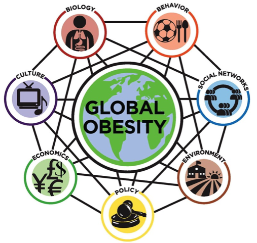
FIGURE 2.2: Obesity as a complex system: http://goo.gl/m2Qq13

2.4 Systems Thinking and Models

Once we take the systems perspective, we have to deal with many components that interact in potentially complicated ways. This makes study and analysis complicated, especially if we are trying to gain insights into the causal and mechanistic connections between system components and their effect on outcomes of interest. While a qualitative, conceptual model (e.g. the one shown in Figure 2.2) often provides some qualitative understanding, it is limiting. It is for instance almost impossible to gain a good quantitative understanding how changes in certain conditions and components of a system lead to changes in outcomes of interest by relying on conceptual approaches alone. If we want to go beyond qualitative and move toward a quantitative understanding (i.e. ‘increasing the tobacco tax by X% will reduce smoking-related health care costs by Y%’), we need quantitative, i.e. mathematical or computational, models. There are many different types of such models one can use. The following provides a - very brief - overview of different modeling approaches.

2.4.1 Phenomenological (statistical) Models

A huge class of models consists of what is usually refered to as statistical models. In the context of this discussion, I prefer to label them phenomenological models, but that terminology is rarely used. The idea behind the statistical/phenomenological approach is to use a mathematical or computational model to study if there are any patterns between the components of the system and the outcomes of interest.

For instance, a linear regression model investigates if there is a pattern between input (system components or other measurable quantities that are part of the system) and an outcome of interest that can be approximated by a linear function. More complicated statistical models exist, some go by the name of machine learning methods. All of these models try to determine if there are patterns between inputs and outputs of interest in the data. Some of the more complicated models allow for interactions between system components (inputs, predictors, variables). Figure 2.3 gives an illustration of 2 simple phenomenological models fit to some data.

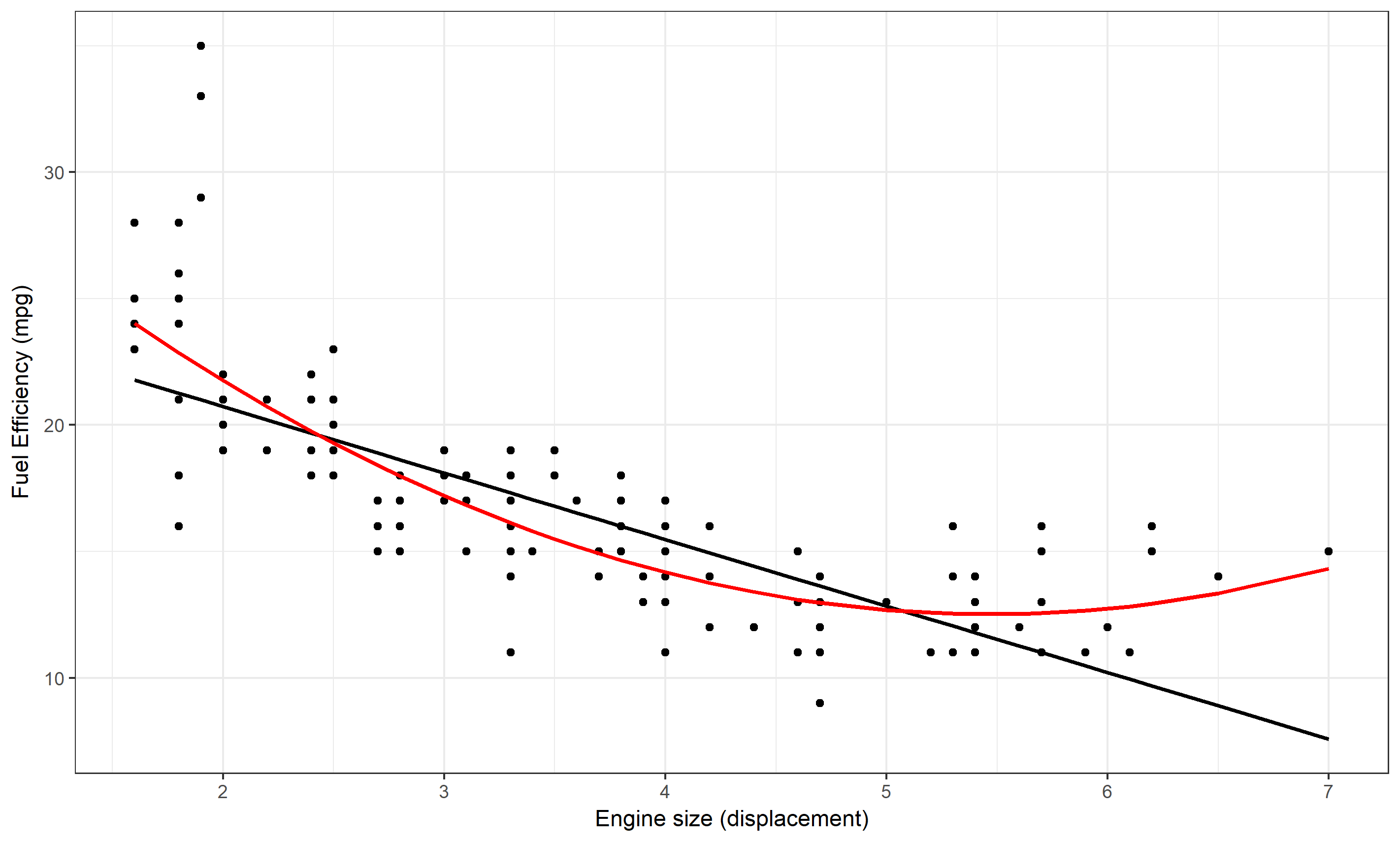
FIGURE 2.3: Two phenomenological models, a linear and quadratic equation, fit to data. The data and model suggest that there is a clear pattern of decreasing fuel efficiency as engine size increases. It seems the pattern is somewhat better described by the quadratic model.

One feature these phenomenological models have in common is that they do not try to describe the mechanisms of interactions within the system that lead to the observed patterns. For instance, if we find that the relationship between the number of cigarettes smoked per day and the 5-year risk of lung cancer can be approximated by a sigmoid function, it does not tell us much about the mechanisms leading from smoking to lung cancer.

2.4.1.1 A few more comments regarding phenomenological models

The big category that I call phenomenological models can of course be further divided. A useful division and way of thinking is between fairly simple models based on some underlying statistical theory and used to explain relations between some factors and some outcome, versus more complicated, often “black-box” type of models that are mainly used to predict an outcome based on some inputs. The former area is the topic of most “classical” statistical work, while the latter often goes by names such as machine learning, data mining, or similar. While simple models are sometimes considered explanatory and can provide clues toward causal links between some inputs and some outputs, they still do not provide insights regarding the mechansisms, which distinghuishes all of these models from mechanistic ones. For more information on the explanatory vs. predictive approach to model uses, the papers (Shmueli 2010) and (Breiman and others 2001) are good starting points.

2.4.2 Mechanistic Models

A class of models that is complementary to the just discussed phenomenologica models are mechanistic models, which explicitly - albeit usually in very simplified form - try to model the mechanisms of interaction among system components. These models are commonly used the hard sciences and engineering. For instance the mathematical equations describing the movement of fluids or electromagnetic fields, or computer simulations of airplane engines, are based on such mechanistic models. The advantage of these kinds of models is that they potentially provide better and deeper understanding of the system. The main disadvantage is that we already need to know (or at least assume) a good bit about how the components interact for us to be able to build such a model. If we have no idea what mechanisms are at work in our system of interest, we cannot build a mechanistic model. Because of that, areas that are currently less well understood (e.g. the functioning of the stock market or the working of brains) are currently not well described by mechanistic models.

One advantage of a mechanistic model is that once it is specified and built, it can be investigated (either mathematically, or more likely through computer simulations) without the need of additional data. For instance, our ability to build decent models capturing the salient features of hurricane dynamics allows us to forecast the storm trajectory. An example of a simulation for a simple mechanistic model is shown in Figure 2.6.

Both phenomenological (statistical) and mechanistic models are useful tools with distinct advantages and disadvantages. Deciding which one to use depends on the question and study system. In this book, we focus on mechanistic models, which try to represent an explicit, simplified description of the system of interest.

2.4.3 Dynamical Models

While the interactions of components always have some implicit time factor, the explicit consideration of time in models is not always needed. Consider this example: We could build a model to study how a change in tobacco taxes might lead to changes in healthcare costs in a given state. Of course, time is present in this system: First we change the taxes, and then we look at changes in costs over some time frame. However, when studying this system, one usually doesn’t need to consider an explicitly time-dependent dynamic. Instead one looks at 2 scenarios: Taxes 1 & Costs 1 versus Taxes 2 & Costs 2. It is usually not necessary to model or simulate the chain of events leading from tax change to cost change while explicitly accounting for time.

However, often the interactions of components that make up a system occurs over time and the temporal component needs to be included. We often want to know how certain changes to the system (e.g. interventions) lead to changes in outcomes through a dynamical/time-dependent chain of events. This leads to dynamical models. For infectious diseases, we most often have some underlying dynamics that we need to take into account (e.g. an ongoing outbreak) and on top of which we might want to implement some interventions. Therefore, the dynamical perspective is generally used.

We can illustrate this dynamical perspective in an abstract way by extending the epidemiological triangle. Figure 2.4 shows the components and the interactions of the triangle changing over time.

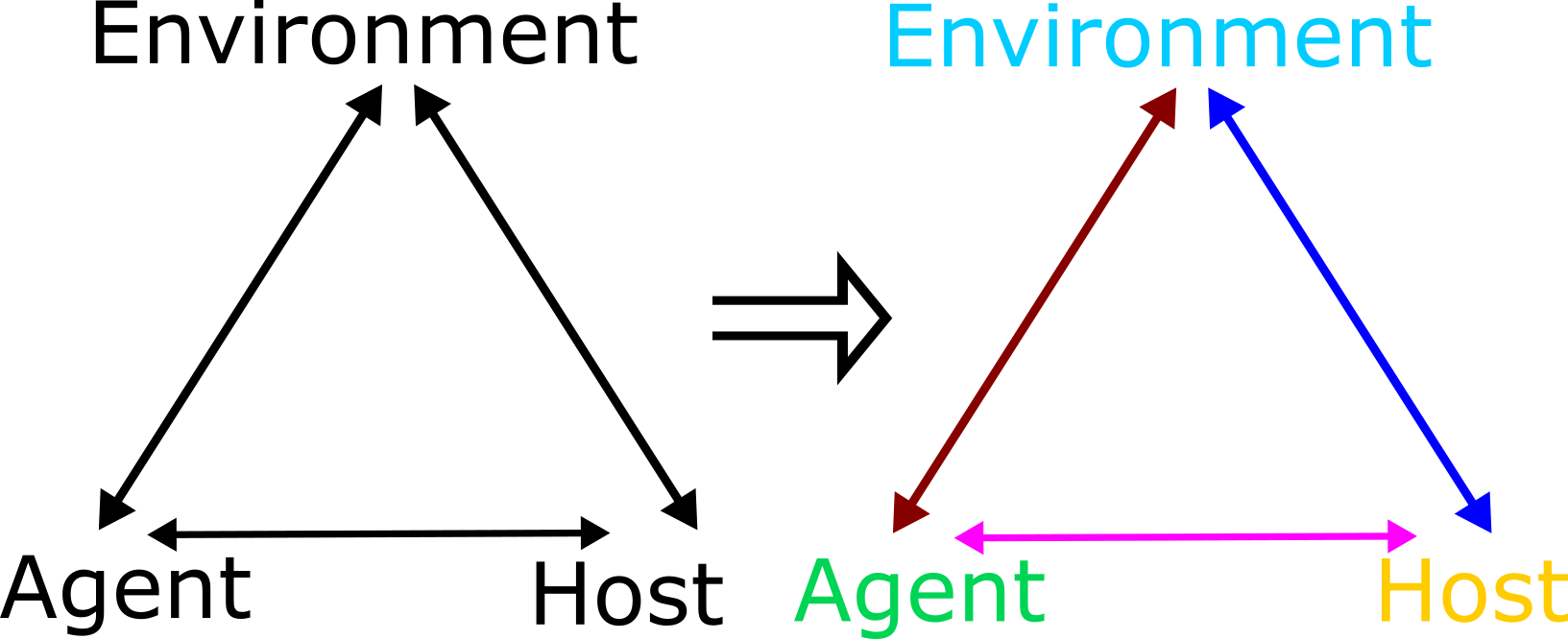
FIGURE 2.4: Dynamic Epidemiological Triangle. Interactions between agent, host and environment change explicitly with time - indicated by the different coloring for each component and interaction.

A more specific example of a simple dynamical model showing changes over time is shown in Figure 2.6.

Mechanistic models are especially well suited to describe dynamical systems and are therefore the primary choice for the study of complex dynamical systems.

2.4.4 Types of Dynamical, Mechanistic Models

When building mechanistic, dynamical models based on a systems approach, there are two main approaches. In one approach, the model is made up of individuals (who are sometimes called agents) and thus these types of models are called agent based or individual based models. The agents/individuals - which are often but not always are humans - interact with each other. Each agent has certain properties and undergoes certain actions. The interactions of all the agents lead to potentially interesting and complex dynamics.

Schelling’s segregation model (see e.g. this video ) is a nice example of such an individual based model. Models and approaches that consider individuals connected through networks of contacts are a type of individual based model that is particularly important for infectious diseases. We will discuss such network concepts in a later chapter.

Another approach simplifies the system by not tracking every individual, but instead only keeps track of total numbers in certain states. For instance, for an ecological model, we might track the total numbers of predators and prey (e.g. wolves and sheep). The resulting model is much simpler. If we had a population of a 100, 1000 or 10,000 wolves or sheep, we would need to keep track of as many individuals. If we only keep track of the total number of individuals, we only need to track how the numbers in each compartment (here wolves and sheep) change - no matter how large our population. Those models, which only track total numbers of individuals, are called compartmental models.

While these compartmental models are obviously simplifications of the real system, they often retain enough of the model complexity to allow us to study the system in detail. Because of this, the majority of models used in infectious disease epidemiology are still these types of compartmental models. Both the DSAIDE R package and the example models shown in this book focus on such compartmental models. The only exception is the chapter on networks.

2.5 Systems approaches in ID Epidemiology

While concepts such as the epidemiological triangle acknowledge that interactions between components are important and determine the behavior of a system, in practice the standard epidemiological approach, based on classical study designs such as cohort, case-control and the randomized trial does not consider system interactions. Indeed, a hallmark assumption of these study designs is that individuals are independent. E.g. the chance that someone in a cohort study has the outcome of interest does not affect the chance of someone else having the outcome. That works well for non-transmissible diseases, and to some extent for transmissible/infectious diseases (we’ll use the term infectious disease in the following, mostly meaning diseases that are also transmissible), as long as there are no interactions (i.e. contact that could lead to transmission) between study subjects. Accounting for interactions between hosts is required to understand important infectious disease concepts such as population level immunity thresholds, critical community size, or indirect effects of interventions. This, in turn, leads to a systems approach that explicitly allows for interactions between hosts.

On the research side, the importance of such interactions has long been appreciated and is at the core of the infectious disease modeling paradigm, where one builds and analyzes a system of interacting components (e.g. susceptible and infected hosts). Model based system approaches have a long history in infectious disease epidemiology Blower and Bernoulli (2004). The importance of computational methods for the study of infectious diseases continues to increase. In this book, we approach infectious diseases from such a systems thinking perspective, without delving too deeply into the mathematical and computational aspects of the topic. If you are interested in building your own models, the books (Matt J. Keeling and Rohani 2008; Vynnycky and White 2010) are good starting points.

2.6 A Basic Infectious Disease Systems Model

For infectious disease models, the simplest dynamical systems model keeps track of the total number of individuals who are susceptible, infectious and removed/recovered (the so-called SIR model). This model is a compartmental model, i.e. we place individuals into distinct compartments, according to some characteristics. We then only track the total number of individuals in each of these compartments. In the simplest model, the only characteristic we track is a person’s infection status according to 3 different stages/compartments:

• S - uninfected and susceptible individuals.
• I - infected and infectious individuals.
• R - removed (recovered and immune or dead) individuals. Those are individuals that do not further participate, either because they are now immune or because they died.

When talking about the quantities that are tracked in each compartment, you will see both the term host(s) and individual(s) used interchangeably. While we most often think of human hosts, the hosts can be any animal (or plants infected by viruses or bacteria infected by phages, etc.). Sometimes, a compartment might track a quantity such as pathogen load in the environment.

In addition to specifying the compartments of a model, we need to specify the processes/mechanisms determining the changes in each compartment. Broadly speaking, some processes increase the number of individuals in a given compartment/stage and processes that lead to a reduction. Those processes are sometimes called inflows and outflows.

For our system, we specify only 2 processes/flows:

1. A susceptible individual (S) can become infected by an infectious individual (I) at some rate (for which we use the parameter b). This leads to the susceptible individual leaving the S compartment and entering the I compartment.
   
2. An infected individual dies or recovers and enters the removed (R) compartment at some rate. This is described by the parameter g in our model.

In general, the entities that change (that vary) in our system (here the number of individuals in compartments S, I and R) are called variables and are each represented by a compartment. In contrast, the quantities that are usually assumed fixed for a given system are called parameters. For the model above, those are the infection rate b and the recovery rate g. This is not a fixed rule, though, and sometimes parameters can be allowed to vary.

The SIR model is very basic, but it still has the hallmark of a complex system. Specifically, there is an interaction between components, namely the I component interacts with the S component, namely infected individuals can infect susceptibles.

For compartmental models (and often other types of models), it is useful to show a graphical representation of the compartments and processes included in the model. For compartmental models, such a diagram/figure is usually called a flow diagram. Such a diagram consists of a box for each compartment, and arrows pointing in and out of boxes to describe flows and interactions. For the simple SIR model, the flow diagram is shown in Figure 2.5.

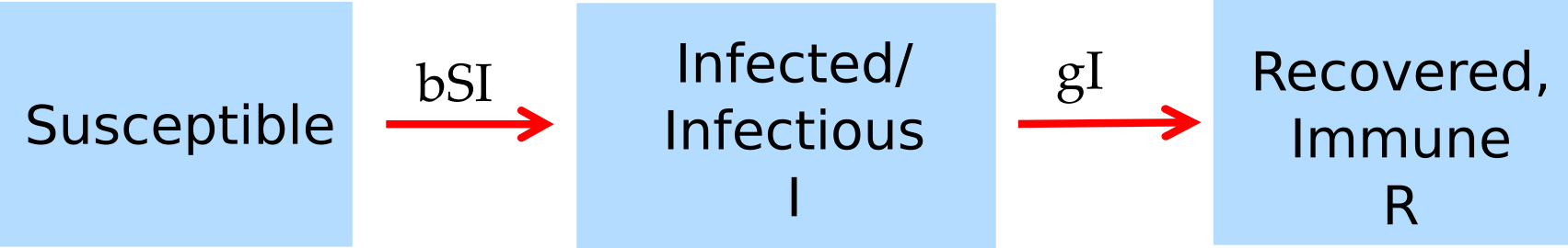
FIGURE 2.5: Flow diagram for the simple SIR model.

To study a specific ID and scientific question, one needs to use a model that approximates the real system one is interested in reasonably well, and one needs to choose values for the model parameters and starting conditions such that they match the specific system one wants to study. We’ll return to that idea throughout this book.

We can implement the flow diagram as a computer model, for instance by formulating it as the set of ordinary differential equations shown below, and then implementing those on a computer to simulate an outbreak. Figure 2.6 shows such a simulation.

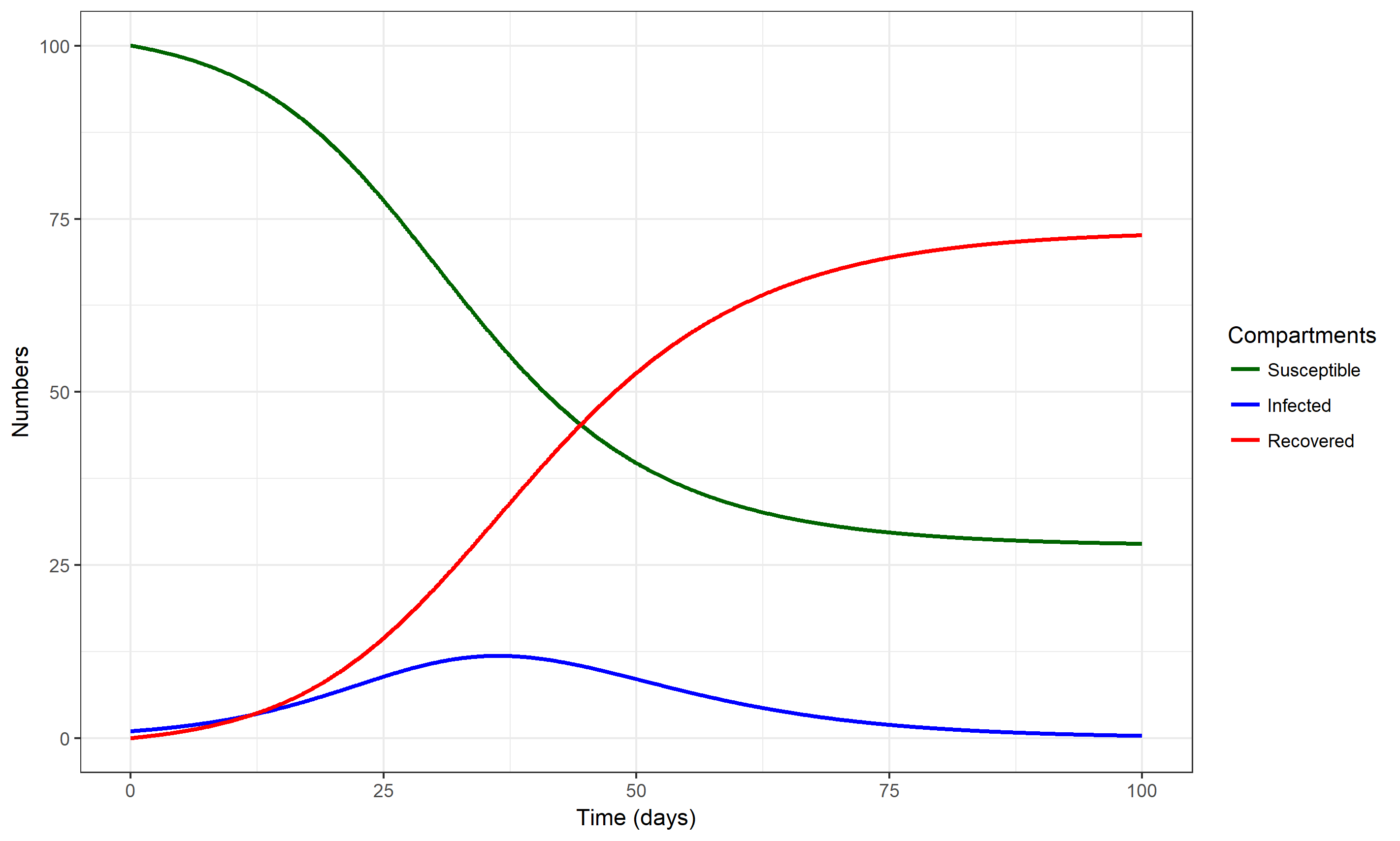
FIGURE 2.6: An outbreak simulation using the simple SIR model. Values for parameters are chosen as b=0.0025/days and g = 1/(7 days). The starting conditions for each compartment are set to S=100, I=1, R=0.

For some more further information on compartmental models in epidemiology, check out this Wikipedia article. We will also discuss many variants of these type of compartmental models in further chapters.

2.6.0.1 Notes

Typically, you will find infectious disease models referred to, or named, according to the compartments therein considered. For example, the aforementioned basic infectious disease model with compartments for Susceptible, Infected, and Removed persons is often plainly called the SIR model. This naming convention also partially extends to include some of the more prominent processes simulated. In an SIS model, there are only two compartments: Susceptible and Infected. So rather than an additional compartment, the second “S” refers to the process governing the flow of infected individuals back into the susceptible compartment following infection; this mimics repeated infections or infections for which no protective immunity is developed.

Unfortunately, there are no strict rules concerning the naming of variables and parameters. Compartments (e.g. SIR) tend to be labeled very similarly by different researchers, while parameter labels are much more variable. I’m trying to be consistent in this book, though I might mix it up occasionally. For this book, I decided to stick with letters from the English alphabet, but you can often find people use Greek letters for parameters (e.g. \(\beta\) instead of b for the transmission parameter). Always check carefully what the definition and meaning of each variable and parameter are.

Here and in other places, I am often sloppy and use the word “infected” even if more precisely, I mean “infected and infectious.” You will find such somewhat sloppy terminology throughout the literature. Individuals who are infected but not infectious are often given their own compartment and label, e.g. they are called “exposed” or “latent” - see chapter 3 for more on this. So when you read infected throughout this book (and in most other places), assume it means ‘infectious’ as well, unless otherwise stated.

2.6.0.2 Model Implementation

If one wants to study any model in detail, one needs to implement it either in the form of a mathematical or a computer model (or both). For compartmental models, the most common way of implementation is writing the model as a set of ordinary differential equations and implementing those in some computer language. This book shows sets of ODE equations for most of the discussed models, but a detailed understanding of these equations is not required to understand the different topics we discuss. For the model described above, the equations look like this: \[\dot S = -bSI\] \[\dot I = bSI - gI\] \[\dot R = gI\]

We are using the usual short-hand notation, where a dot over a variable means its derivative (its change) with respect to time. In all the models we consider, we always only consider changes with respect to time (the dynamical aspect of the model). The left side indicates which variable changes, and the right side indicates how it changes. Anything with an (usually not shown) positive sign on the right side describes a positive change, i.e. an inflow into the specified compartment, thus increasing the number in that compartment. Anything with a negative sign indicates an outflow out of that compartment.

2.7 Summary and Cartoon

This chapter provided a brief introduction to the concept of systems thinking and how modeling is used to study complex systems. We briefly looked at a simple infectious disease systems model, the famous SIR model.

FIGURE 2.7: Not every diagram helps to understand a complex system. Source: xkcd.com.

2.8 Exercises

• If you haven’t done already, install R, RStudio and the DSAIDE R package. See (Handel 2017) for an overview and quick-start guide for DSAIDE.
• Work through the tasks for the ID Dynamics Introduction DSAIDE app.
• Contemplate on your experience with the ID Dynamics Introduction DSAIDE app. In which way does it capture the ‘dynamical systems’ perspective? Did you find any behavior of this - arguably very simple - infectious disease model to be complex? How/why?
• Read the paper “Systems Science Methods in Public Health: Dynamics, Networks, and Agents” by Luke & Stamatakis (Luke and Stamatakis 2012). Come up with 2 systems that you consider complex in the realm of public health or biomedicine (other than those mentioned in the paper). Explain what makes them complex. Also, come up with 2 systems that you consider not complex and explain why you think of them as not complex.

2.9 Further Resources

• The paper “Why Model?” by Joshua Epstein (Epstein 2008) provides a nice, short discussion of the purposes of models. Other general introductory discussions of systems thinking and model use are (R. M. May 2004; Chubb and Jacobsen 2010; Garnett et al. 2011; Basu and Andrews 2013; Gunawardena 2014; Homer and Hirsch 2006; Peters 2014; Sterman 2006).
• Several introductory papers on infectious disease modeling can be found in e.g. (M. J. Keeling and Danon 2009; Heesterbeek et al. 2015; Lessler et al. 2016; C. Jessica E. Metcalf and Lessler 2017).
• While the dynamical systems approach has been applied to infectious diseases for a long time, it is starting to be used more frequently in other areas of public health. Some recent references on that topic are e.g. (Ness, Koopman, and Roberts 2007; Sánchez-Romero et al. 2016).
• If you want to learn more about individual based models, see e.g. (Railsback and Grimm 2011).

2.10 References