Chapter 10 Host Heterogeneity
10.1 Overview and Learning Objectives
In this module, we will briefly discuss the idea that hosts differ in characteristics that are important with regard to ID dynamics and control.
The learning objectives for this chapter are:
- Know the most common host characteristics that lead to heterogeneity
- Understand how heterogeneity might impact ID dynamics
- Evaluate the need to account for heterogeneity depending on setting
- Understand how different types of heterogeneity affect ID control
10.2 Introduction
So far, we tracked hosts concerning their infection status (susceptible, infected, symptomatic, recovered, etc.). We assumed that hosts are similar enough with regard to any other characteristics that might matter for ID dynamics and control that we did not have to consider them. For instance, we did not account for age, sex, pre-existing conditions or any other such potentially differentiating detail among hosts.
That approach is of course at best a decent approximation and at worst completely wrong. Many characteristics affect how an ID interacts with a host. For instance, for many ID, children and the elderly are more likely to get infected and might suffer more severe symptoms. For other ID, only specific groups are affected. For instance, only sexually active individuals are at risk of contracting a sexually transmitted infection (ignoring for a moment less common transmission routes such as blood transfusion for HIV). We will discuss some of these differences/heterogeneities between hosts and how they affect ID transmission and control in this module.
10.3 Types of Host Heterogeneity
We generally only care about differences in hosts as they relate to the infectious disease process. Consider a simple - maybe silly - example: Almost no infectious disease study (none that I know of) cares about a person’s hair color. That’s because this characteristic has - as far as we are aware - no effect on the interaction of host and ID. On the other hand, a fundamental feature that affects many IDs is age. Therefore age often needs to be taken into account when studying IDs. Other important more broad categories such as genetics and behavior can also affect ID infection and spread.
Some host characteristics might only have an impact on a single component of the ID, e.g., the level of susceptibility to infection. Other host differences can affect multiple components, e.g., a person with numerous sexual partners is more likely to contract an STI, and if they are infected, they are also more likely to transmit an STI.
10.3.0.1 Host Heterogeneity Examples
Several famous examples show how differences in genetics can impact ID. For instance, persons with a certain mutation of the CCR5 co-receptor on T-cells are much less likely to get infected with HIV. Similarly, persons with a particular mutation in the FUT2 gene are much less likely to get infected with norovirus. It is probable that there are genetic differences for almost any ID that influence the probability of getting infected, the severity of symptoms, and the duration and amount of shedding.
10.4 Heterogeneity in Transmission: Core Groups
To study ID transmission dynamics, differences in the potential and ability of individual hosts to spread an ID are obviously of great importance. This idea of heterogeneity in transmission has been studied in several contexts and under different names. One of the first was the concept of a core group introduced to explain the persistence of gonorrhea in the 1970s (see (Yorke, Hethcote, and Nold 1978)). Core groups are subgroups in which transmission is higher compared to other groups. For many STI, transmission in the general population is low enough that the reproductive number is below 1. The question then is, why does that not lead to the extinction of the ID? The core group concept provides a reasonable explanation. Where a small but defined population of individuals maintain the ID with a reproductive number that is greater than 1. Infections spread from this group to those in the general population allows the ID to persist in the general population with a reproductive number less than 1.
Once we have identified that different groups have different transmission behavior, it also becomes necessary to understand how individuals belonging to one of the groups interact with people of the other groups. Often called the mixing pattern between groups. We are most interested in the mixing and contact patterns that facilitate transmission of the ID under consideration. For instance, it is well known that humans tend to have more contacts with others of the same age, e.g., children predominantly contacting other children. This is called assortative mixing, and such age-specific mixing is important for the transmission of many respiratory diseases. The opposite is disassortative mixing. For instance, for STI, most mixing occurs between individuals from the opposite sex (and there are also more contacts among individuals of similar age). Therefore, for STI, mixing with regard to gender can be considered disassortative. However, it is also known that people who engage in risky sexual behavior (e.g., more partners per year) tend to have more contacts with others that engage in similar risk behavior, thus with regard to transmission and infection risk, STI often show assortative mixing. If there is no mixing preference, it is called random mixing. The random mixing assumption is made implicitly in any model that does not account for contact/transmission heterogeneity, e.g., the basic SIR model assumes random mixing and contact patterns between susceptible and infected, independent of any other characteristic. Determining the mixing patterns between individuals is important but also difficult. For some research in that area, see, e.g. (Edmunds et al. 2006; Mossong et al. 2008).
10.5 Heterogeneity in Transmission: Superspreaders
An equivalent concept to that of the core group, but applied to individuals, is known by the term superspreaders. Superspreaders are individuals who spread/transmit an ID much more than the average infected person. It turns out that for most ID, the number of secondary transmissions produced by the average infected person is not too meaningful. Such a measure would be a good description if the distribution of secondary infections were close to normal (or Poisson), with most infected individuals infecting similar numbers of others. However, what is often observed is a heavily skewed distribution, with most individuals infecting none or only a few others, and a few individuals infecting many others (Galvani and May 2005).
10.6 Heterogeneity and The Reproductive Number
If we have multiple host types, we need to extend the idea of the reproductive number. While it is possible to compute a reproductive number for the overall population, this quantity might not tell the full story. Instead, we might want to look at the reproductive number for subsets of the population, for instance for the general population (non-superspreaders) and core groups (the superspreaders). If one wants to compute an overall reproductive number, one needs to account for the population heterogeneity by including a measure of the variability of contacts in the equation for the reproductive number. See, (Robert M. May, Gupta, and McLean 2001) for a discussion of this topic.
10.7 Heterogeneity and ID control
Heterogeneity among hosts concerning their susceptibility, infectiousness, and severity has direct implications for control. If we know who is most likely to transmit, who is most likely to have a severe case of a disease, and who is most likely to catch an ID in the first place, we can implement targeted control strategies. For instance, instead of vaccinating people at random, we could target those that are most vulnerable to getting the ID, or those most likely to infect others if they were to get infected. The better we can target the intervention, the more impact they can have, and while also getting more ‘bang for our buck.’
10.8 Modeling Heterogeneity
The basic concept of including host heterogeneity in models is relatively straightforward. We stratify the population according to the characteristic we want to take into account. For instance, instead of lumping everyone into susceptible-infected-recovered categories, we can track males and females, or children and adults, separately. Figure 10.1 illustrates this.
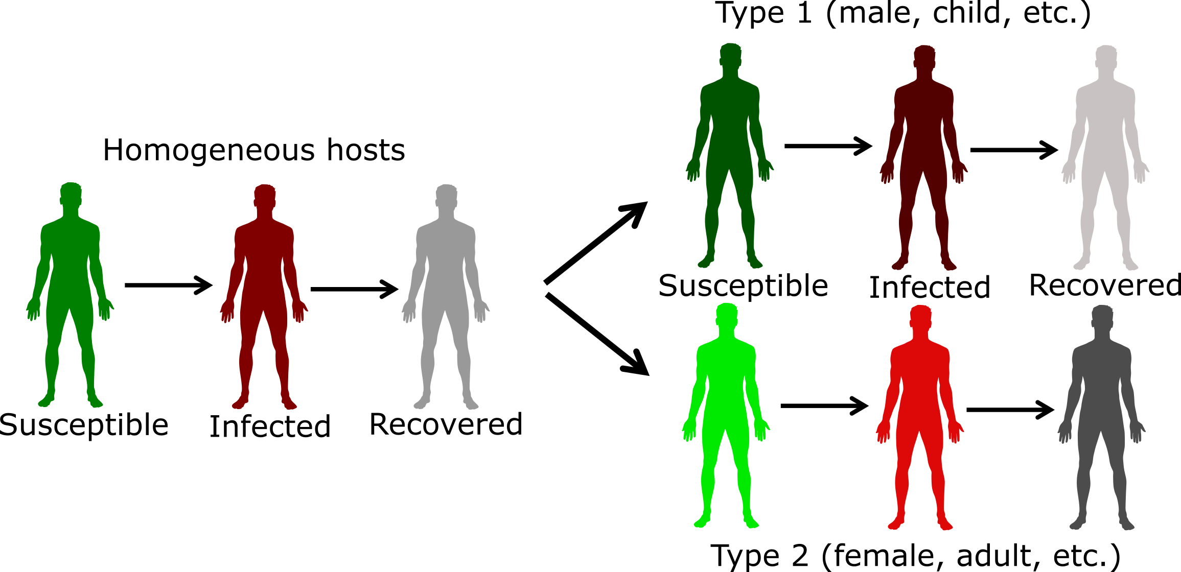
FIGURE 10.1: Example of including host heterogeneity in an SIR model.
The challenges with including more details in the model are not conceptual but are instead logistical and potentially technical. Bigger models are harder to formulate, implement, and analyze. Additionally, we need estimates of model parameters with regard to the stratifying characteristics, which are often hard to get. Because of that, it is often best to start with a simple model, and slowly introduce host characteristics as they are deemed relevant to the ID setting, and question one wants to address.
At some point, if we want to include a lot of detail, it might be worth switching the modeling framework. For compartmental models, hosts are grouped according to characteristics. As we want to track more characteristics, the number of compartments we need to include increases. If the basic model has C compartments/variables, P parameters, and we model N subpopulations, we have C x N equations and at least P x N (or more) parameters. For instance, if we had a basic SEIR model (4 compartments), and wanted to track males and females in 4 different age groups, we had 4 x 2 x 4 = 32 compartments. If we had additional compartments to follow say vaccination or treatment status, one could end up with more than 50 compartments, sometimes even going into the hundreds.
Once the number of compartments gets too large, it might then be worth deciding to stop using compartmental models and instead switch to a type of model that is called agent or individual-based model (ABM/IBM). In such models, the individual host is modeled and tracked. We can give everyone as many different characteristics as we want. This makes the model very flexible and potentially very realistic. The downside of these ABM is that they tend to be more complicated than compartmental models, are generally much harder to code, and often take a long time to run, especially if one wants to model a large population. Further, for detailed models, lots of parameter estimates are needed, and they are often not available, leading to potentially large uncertainty in model predictions. Also, it ’s hard to make any statistical inference with ABM. Because of these disadvantages, the compartmental modeling framework is still the most frequently used and a good starting point for most situations and questions. For IDs where we know a lot and want detailed predictions (e.g., influenza), ABMs are becoming more common.
10.9 Summary and Cartoon
This chapter provided a brief discussion of host heterogeneity, how to consider it in studies, and its impact on transmission and control. We also discussed how to include heterogeneity into models.
FIGURE 10.2: That is the best heterogeneity cartoon I have - let me know if you know a better one!
10.10 Exercises
- The Host Heterogeneity app in the DSAIDE package provides hands-on computer exercises for this chapter.
- Read the article “Disease spread, susceptibility, and infection intensity: vicious circles?” by Beldomenico and Begon (Beldomenico and Begon 2010). The paper mostly discusses non-human IDs. Find evidence from human IDs for which the different components they discuss (variable host susceptibility, variable infection intensity, feedback circles in the individual/population level) might be applicable.
10.11 Further Resources
- Good further discussions of the superspreader concept can be found in (Galvani and May 2005; J. O. Lloyd-Smith et al. 2005; Stein 2011).
- The impact of host heterogeneity on the reproductive number is for instance discussed in (Robert M. May, Gupta, and McLean 2001), an application to Chlamydia is provided in (Potterat et al. 1999).
- An influential study that collected detailed information on contact patterns using a diary approach is (Mossong et al. 2008).
- General discussions of transmission heterogeneity are given in (Matthews and Woolhouse 2005; Paull et al. 2012).
- Host heterogeneity and control is for instance discussed in (Yorke, Hethcote, and Nold 1978; M. E. Woolhouse et al. 1997).