Decision Trees
Overview
In this unit, we will cover a class of models generally referred to as decision trees.
Learning Objectives
- Understand what tree-based methods are and how to use them
- Know the difference between regression and classification trees
- Know when it might be good to use a tree-based method
- Understand the advantages and disadvantages of single tree model
Introduction
Simple GLMs have the main limitation of capturing only overall smooth patterns relating inputs and outcomes. Higher order terms or interactions must be manually specified. The polynomial and spline models we discussed allow for more flexible patterns, at the cost of more potential overfitting and also reduced interpretability. Another class of models that allow non-linear relation between inputs and outcomes are based on decision trees. In general, a decision tree is a tree-like structure that helps you make decisions. In machine learning, there are specific methods to build those trees. Decision trees can be used for continuous outcomes, in which case they are called regression trees or for categorical outcomes, in which case they are called classification trees. The umbrella term Classification and regression trees - or CART for short is also often used to mean the same as decision trees.
Basic tree models have the advantage of being fairly easy to understand and use, even by non-statisticians. Trees can deal with nonlinear relations between predictors and outcome, they easily accomodate more than two categories for classification, and they can handle predictors that have missing values.
Tree Examples
The following shows a tree from Afonso et al. 2012, which is a study led by one of my colleagues Mark Ebell to determine if there are simple decision rules that can determine if a person has an influenza infection or not.
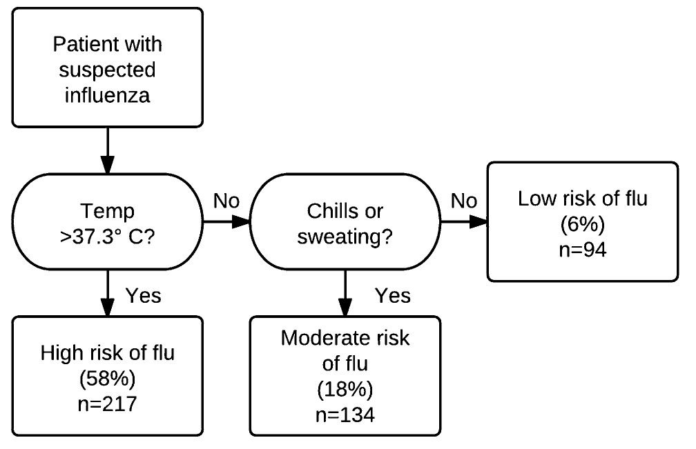
As you can see, this is a very simple model that is very intuitive and could be easily understood by physicians and other laypeople. The tree is used here for classification, with a binary outcome (presence/absence of flu).
The next example is a tree used for a regression problem to predict/model a continuous outcome.
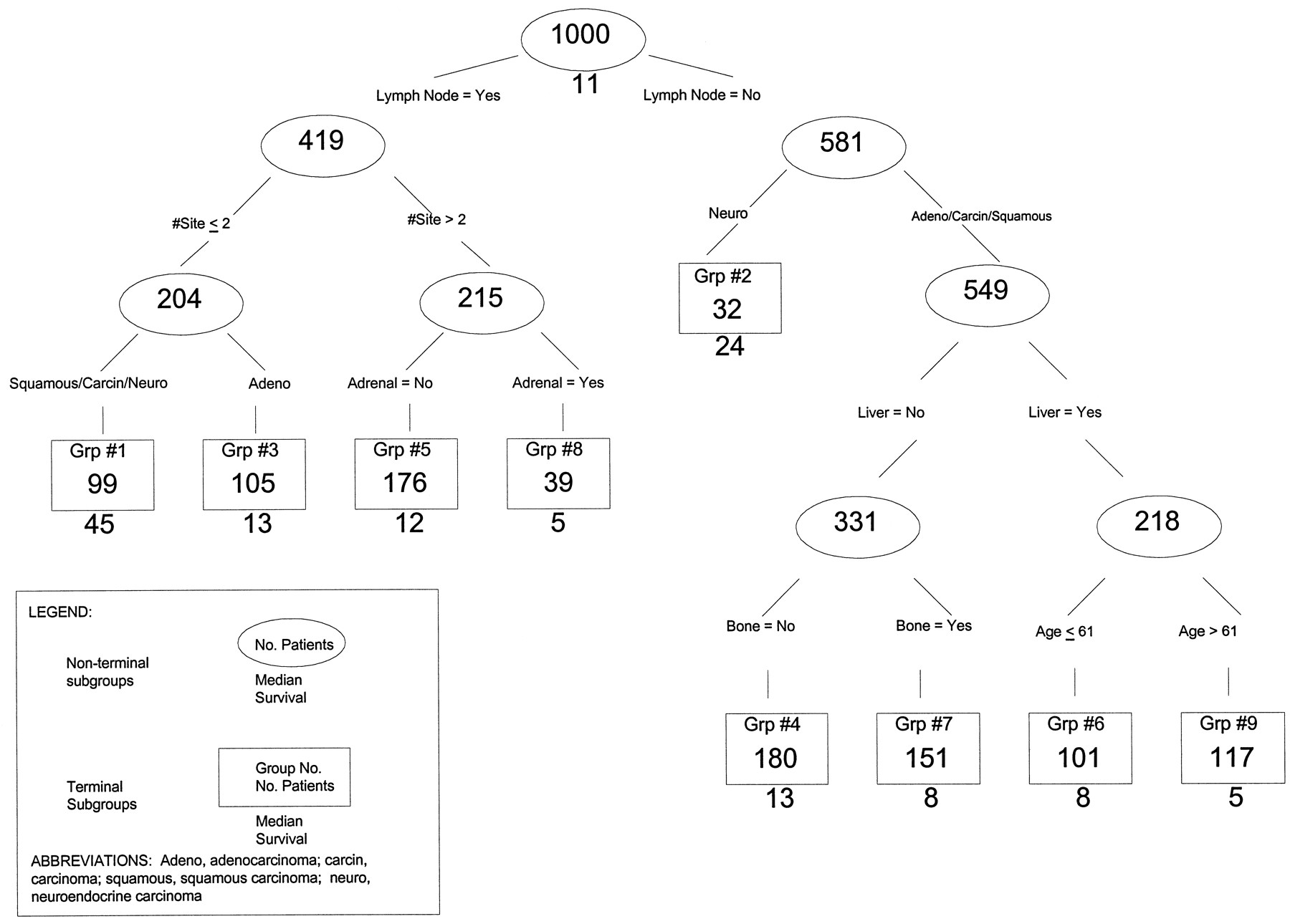
In this study, the authors tried to determine the survival time of patients who had cancers with certain characteristics. The tree was used to group individuals, and for each group the tree/model predicts median survival.
Building trees
The way one computes a tree is a little bit similar in concept to forward selection in a linear model. We start by looking at each predictor. We take the tree, which, when the outcome is split at some value of that predictor, leads to the best (cross-validated) performance increase in the model (e.g., lowest SSR/RMSE or highest Accuracy/F1 score). Let’s say we want to predict BMI, and our performance measure is RMSE of predicted value from the true outcome. The null model using no predictors gives us some value for the RMSE. We then try each predictor (let’s say we have exercise, calories, age, sex) and find that if we use exercise and assign everyone who exercises more than 23min per day one BMI value, and everyone who exercises less than 23min another BMI value, we get the best reduction in RMSE we could get (across all predictors and possible cut-off values). This is our first split using the exercise predictor at 23min. We now have a tree with one root and 2 nodes (in this case, they are leaves, which is the name for the terminal nodes).
We now take each leaf and run through all predictors again including the one we just used and see which predictor split at some value will further improve model performance. Let’s say we find that for those exercising more than 23min, we can split by sex and get 2 new BMI values, one for males exercising >23min and one for females exercising >23min, which gives the maximum reduction in RMSE. Similarly, we find that for the <23min exercise people, splitting at 1500 calories a day is best. We now have a tree with a root, 2 internal nodes, and 4 terminal nodes.
We keep building the tree in this way until some criterion is met (e.g., no more than n observations in a given leaf, no further increase in performance). Note that in this procedure, some predictors may never enter the model. In that way, a tree performs an automatic subset selection, i.e., the algorithm might decide to not include predictor variables it doesn’t find useful. Also, any predictor could be used more than once.
Algorithms that implement the tree building routine differ in their details, which is why you will see many different options in both mlr and caret. In general, if you have a good signal in your data, any algorithm should pick up on it.
Since trees have a tendency to overfit, it is common to regularize them by including a penalty for tree size. For instance, if we were to minimize SSR/RMSE, we would add a penalty to the cost function, C, to get
\[C = SSR + \lambda T, \]
where T is the number of leaves of the tree. More leaves means a larger tree, which is being penalized. The tuning parameter \(\lambda\) needs to be determined using parameter tuning or model training. Reducing a tree in this way is also called pruning.
Fast and frugal trees
While trees are fairly simple to understand, sometimes, especially if there are many branching points, a complex decision tree might still not be suitable in practice. Further, even with regularization, trees might overfit. There is a type of tree, called fast and frugal tree (FFT), which can potentially help with both aspects. The difference between a regular tree and a FFT is that for the FFT, at each split/decision point, at least one of the splits needs to end in a terminal node. Check e.g. the example diagrams shown in the FFT Wikipedia article to see what this means. This constraint makes the trees often simpler and thus easier to implement in practice (e.g. by a doctor) and they might also be more robust, i.e. their performance on future data might be better than a larger tree. Disadvantages of FFT are that sometimes they might be too simple and thus not perform as well as a full tree, and they only work for binary outcomes.
A very nice R package called FFTrees implements FFT (and automatically compares their performance to regular trees and some of the tree based methods discussed below). You can find more about this R package in the FFTrees documentation.
Advantages and disadvantages of tree models
A great feature of trees is that they are relatively quick and easy to build and especially easy to understand. They can easily be communicated to and used by non-experts (e.g., doctors, other decision-makers). As such, trees (sometimes called decision diagrams or other names) are common in many fields. As mentioned, trees are also able to handle missing data in predictors, and they are often reasonably robust in the presence of collinear or near-zero-variance predictors since trees tend to use one of the variables and ignore the others. Tree models also tend to excel at inferring the presence of nonlinear interactions between variables. Often trees don’t need predictors to be standardized either.
The main disadvantage of trees is that they usually have reduced performance compared to other models. Thus, if a simple, interpretable model is the primary goal, trees are ideal. If instead, a high-performance predictive model is the goal, trees are rarely the best choice.
Further information
R2D3’s excellent interactive tutorial gives a very nice, visual introduction to machine learning in general and trees in particular. It covers and nicely illustrates some of the topics discussed here, as well as topics discussed in previous units. In part 2 of the tutorial the authors discuss overfitting. I strongly recommend you check it out, even if you just skim through it. It is fun and informative!
For more on tree models, see the first part Tree-based Methods chapter of ISLR, the Decision Trees chapter of HMLR.