library('dplyr')
library('ggplot2')
library('here')Scrambling existing data - R
Overview
In this tutorial, we discuss how to scramble existing data to make it “new”.
Learning Objectives
- Be able to generate scrambled data with
Rbased on existing data.
Introduction
If you want to be as close to the original data as possible, you can just take that data and scramble values such that observations become new.
Let’s say you have individuals with different characteristics such as age, height, gender, BMI, etc. By just randomly re-assigning values for each variable to individuals, you create new individuals. Those individuals are not real and thus you minimize potential problems with confidentiality.
Since you are using exactly the same values for each variable as in the original dataset, the distribution for each variable remains the same and is thus very close (in fact, identical) to the real data.
However, a problem with such scrambling is that while you preserve the distribution of each variable, you might break associations. For instance, males are generally taller than females. If you randomly scramble both gender and height without taking into account this potential association, you might end up with a dataset that has a distribution of heights among males and females that is the same. Depending on your goals, this might or might not be a problem.
Another drawback of scrambling data is that you can’t build associations between variables into the data generating process, so you don’t really know what your models should find when they look for patterns. Thus, a big advantage of synthetic data, namely the fact that you know exactly how it was generated, goes away.
In general, I’m not too big a fan of the scrambling approach, but there might be scenarios where this is what you want/need, therefore we should talk about it.
AI help
Since you are working with the real data, you probably don’t want to use AI for this, unless your AI tool operates in a secure environment (e.g., fully on your companies’ servers).
Example
Time for a simple example. You can find the code shown below in this file.
Setup
First, we do the usual setup steps of package loading and other housekeeping steps.
# setting a random number seed for reproducibility
set.seed(123)
Data loading and exploring
We’ll look at some real data from this paper. As is good habit (and should be the standard), the authors (which includes some of us) supplied the data as part of the supplementary materials, which can be found here.
If you want to work along, go ahead and download the supplement, which is a zip file. Inside the zip file, find the Clean Data folder and the SympAct_Any_Pos.Rda file. Copy that file to the location where you’ll be placing your R script.
First, we load the data. Note that the authors (that would be us 😁) used the wrong file ending, they called it an .Rda file, even though it is an .Rds file (for a discussion of the differences, see e.g. here).
The data
#assuming your R script is in the same folder
#rawdat <- readRDS('SympAct_Any_Pos.Rda')
# this is for my setup
rawdat <- readRDS('SympAct_Any_Pos.Rda')
Next, we take a peek.
dim(rawdat)[1] 735 63dplyr::glimpse(rawdat) Rows: 735
Columns: 63
$ DxName1 <fct> "Influenza like illness - Clinical Dx", "Acute tonsi…
$ DxName2 <fct> NA, "Influenza like illness - Clinical Dx", "Acute p…
$ DxName3 <fct> NA, NA, NA, NA, NA, NA, NA, NA, "Fever, unspecified"…
$ DxName4 <fct> NA, NA, NA, NA, NA, NA, NA, NA, "Other fatigue", NA,…
$ DxName5 <fct> NA, NA, NA, NA, NA, NA, NA, NA, "Headache", NA, NA, …
$ Unique.Visit <chr> "340_17632125", "340_17794836", "342_17737773", "342…
$ ActivityLevel <int> 10, 6, 2, 2, 5, 3, 4, 0, 0, 5, 9, 1, 3, 6, 5, 2, 2, …
$ ActivityLevelF <fct> 10, 6, 2, 2, 5, 3, 4, 0, 0, 5, 9, 1, 3, 6, 5, 2, 2, …
$ SwollenLymphNodes <fct> Yes, Yes, Yes, Yes, Yes, No, No, No, Yes, No, Yes, Y…
$ ChestCongestion <fct> No, Yes, Yes, Yes, No, No, No, Yes, Yes, Yes, Yes, Y…
$ ChillsSweats <fct> No, No, Yes, Yes, Yes, Yes, Yes, Yes, Yes, No, Yes, …
$ NasalCongestion <fct> No, Yes, Yes, Yes, No, No, No, Yes, Yes, Yes, Yes, Y…
$ CoughYN <fct> Yes, Yes, No, Yes, No, Yes, Yes, Yes, Yes, Yes, No, …
$ Sneeze <fct> No, No, Yes, Yes, No, Yes, No, Yes, No, No, No, No, …
$ Fatigue <fct> Yes, Yes, Yes, Yes, Yes, Yes, Yes, Yes, Yes, Yes, Ye…
$ SubjectiveFever <fct> Yes, Yes, Yes, Yes, Yes, Yes, Yes, Yes, Yes, No, Yes…
$ Headache <fct> Yes, Yes, Yes, Yes, Yes, Yes, No, Yes, Yes, Yes, Yes…
$ Weakness <fct> Mild, Severe, Severe, Severe, Moderate, Moderate, Mi…
$ WeaknessYN <fct> Yes, Yes, Yes, Yes, Yes, Yes, Yes, Yes, Yes, Yes, Ye…
$ CoughIntensity <fct> Severe, Severe, Mild, Moderate, None, Moderate, Seve…
$ CoughYN2 <fct> Yes, Yes, Yes, Yes, No, Yes, Yes, Yes, Yes, Yes, Yes…
$ Myalgia <fct> Mild, Severe, Severe, Severe, Mild, Moderate, Mild, …
$ MyalgiaYN <fct> Yes, Yes, Yes, Yes, Yes, Yes, Yes, Yes, Yes, Yes, Ye…
$ RunnyNose <fct> No, No, Yes, Yes, No, No, Yes, Yes, Yes, Yes, No, No…
$ AbPain <fct> No, No, Yes, No, No, No, No, No, No, No, Yes, Yes, N…
$ ChestPain <fct> No, No, Yes, No, No, Yes, Yes, No, No, No, No, Yes, …
$ Diarrhea <fct> No, No, No, No, No, Yes, No, No, No, No, No, No, No,…
$ EyePn <fct> No, No, No, No, Yes, No, No, No, No, No, Yes, No, Ye…
$ Insomnia <fct> No, No, Yes, Yes, Yes, No, No, Yes, Yes, Yes, Yes, Y…
$ ItchyEye <fct> No, No, No, No, No, No, No, No, No, No, No, No, Yes,…
$ Nausea <fct> No, No, Yes, Yes, Yes, Yes, No, No, Yes, Yes, Yes, Y…
$ EarPn <fct> No, Yes, No, Yes, No, No, No, No, No, No, No, Yes, Y…
$ Hearing <fct> No, Yes, No, No, No, No, No, No, No, No, No, No, No,…
$ Pharyngitis <fct> Yes, Yes, Yes, Yes, Yes, Yes, Yes, No, No, No, Yes, …
$ Breathless <fct> No, No, Yes, No, No, Yes, No, No, No, Yes, No, Yes, …
$ ToothPn <fct> No, No, Yes, No, No, No, No, No, Yes, No, No, Yes, N…
$ Vision <fct> No, No, No, No, No, No, No, No, No, No, No, No, No, …
$ Vomit <fct> No, No, No, No, No, No, Yes, No, No, No, Yes, Yes, N…
$ Wheeze <fct> No, No, No, Yes, No, Yes, No, No, No, No, No, Yes, N…
$ BodyTemp <dbl> 98.3, 100.4, 100.8, 98.8, 100.5, 98.4, 102.5, 98.4, …
$ RapidFluA <fct> Presumptive Negative For Influenza A, NA, Presumptiv…
$ RapidFluB <fct> Presumptive Negative For Influenza B, NA, Presumptiv…
$ PCRFluA <fct> NA, NA, NA, NA, NA, NA, Influenza A Not Detected, N…
$ PCRFluB <fct> NA, NA, NA, NA, NA, NA, Influenza B Not Detected, N…
$ TransScore1 <dbl> 1, 3, 4, 5, 0, 2, 2, 5, 4, 4, 2, 3, 2, 5, 3, 5, 1, 5…
$ TransScore1F <fct> 1, 3, 4, 5, 0, 2, 2, 5, 4, 4, 2, 3, 2, 5, 3, 5, 1, 5…
$ TransScore2 <dbl> 1, 2, 3, 4, 0, 2, 2, 4, 3, 3, 1, 2, 2, 4, 2, 4, 1, 4…
$ TransScore2F <fct> 1, 2, 3, 4, 0, 2, 2, 4, 3, 3, 1, 2, 2, 4, 2, 4, 1, 4…
$ TransScore3 <dbl> 1, 1, 2, 3, 0, 2, 2, 3, 2, 2, 0, 1, 1, 3, 1, 3, 1, 3…
$ TransScore3F <fct> 1, 1, 2, 3, 0, 2, 2, 3, 2, 2, 0, 1, 1, 3, 1, 3, 1, 3…
$ TransScore4 <dbl> 0, 2, 4, 4, 0, 1, 1, 4, 3, 3, 2, 2, 2, 4, 3, 4, 0, 4…
$ TransScore4F <fct> 0, 2, 4, 4, 0, 1, 1, 4, 3, 3, 2, 2, 2, 4, 3, 4, 0, 4…
$ ImpactScore <int> 7, 8, 14, 12, 11, 12, 8, 7, 10, 7, 13, 17, 11, 13, 9…
$ ImpactScore2 <int> 6, 7, 13, 11, 10, 11, 7, 6, 9, 6, 12, 16, 10, 12, 8,…
$ ImpactScore3 <int> 3, 4, 9, 7, 6, 7, 3, 3, 6, 4, 7, 11, 6, 8, 4, 4, 5, …
$ ImpactScoreF <fct> 7, 8, 14, 12, 11, 12, 8, 7, 10, 7, 13, 17, 11, 13, 9…
$ ImpactScore2F <fct> 6, 7, 13, 11, 10, 11, 7, 6, 9, 6, 12, 16, 10, 12, 8,…
$ ImpactScore3F <fct> 3, 4, 9, 7, 6, 7, 3, 3, 6, 4, 7, 11, 6, 8, 4, 4, 5, …
$ ImpactScoreFD <fct> 7, 8, 14, 12, 11, 12, 8, 7, 10, 7, 13, 17, 11, 13, 9…
$ TotalSymp1 <dbl> 8, 11, 18, 17, 11, 14, 10, 12, 14, 11, 15, 20, 13, 1…
$ TotalSymp1F <fct> 8, 11, 18, 17, 11, 14, 10, 12, 14, 11, 15, 20, 13, 1…
$ TotalSymp2 <dbl> 8, 10, 17, 16, 11, 14, 10, 11, 13, 10, 14, 19, 13, 1…
$ TotalSymp3 <dbl> 8, 9, 16, 15, 11, 14, 10, 10, 12, 9, 13, 18, 12, 16,…So it looks like these are 735 individuals (rows) and 63 variables (columns). A lot of them have names of symptoms and are coded as Yes/No. Some variables are harder to understand, for instance without some meta-data/explanation, it is impossible to guess what TransScore3F stands for. Hopefully, your data came with some codebook/data dictionary/information sheet that explains what exactly everything means. For this specific data set, you can look through the supplementary materials to learn more. We won’t delve into it now, and just pick out a few variables to illustrate the data scrambling process.
Data processing
For simplicity, let’s assume we are interested in just a few of these variables, namely ActivityLevel, Sneeze, Nausea, and Vomit. We’ll select those and look at the first 10 entries.
dat <- rawdat |> dplyr::select("ActivityLevel","Sneeze","Nausea","Vomit")
head(dat,10)
ActivityLevel Sneeze Nausea Vomit
1 10 No No No
2 6 No No No
3 2 Yes Yes No
4 2 Yes Yes No
5 5 No Yes No
6 3 Yes Yes No
7 4 No No Yes
8 0 Yes No No
9 0 No Yes No
10 5 No Yes NoData Scrambling
Now we’ll scramble the data. I’m doing this here with a simple loop. I’m looping through each variable, and I sample from the old values without replacement, which basically just rearranges them. There are computationally faster and more concise ways of doing this, but the loop makes it hopefully very clear what’s going on.
# define a new data frame that will contain scrambled values
dat_sc <- dat
Nobs = nrow(dat) #number of observations
# loop over each variable, reshuffle entries
for (n in 1:ncol(dat))
{
  dat_sc[,n] <- sample(dat[,n], size = Nobs, replace = FALSE)
}

head(dat_sc,10)
ActivityLevel Sneeze Nausea Vomit
1 8 No No No
2 5 No No No
3 0 Yes No No
4 3 No Yes No
5 5 No Yes No
6 5 Yes No No
7 1 Yes No No
8 3 Yes No No
9 8 Yes No No
10 6 Yes Yes NoThe first 10 entries look different, so that’s promising.
Comparing old and new data
Now let’s see if things worked. First, we summarize both the old and the new data. We should see that they are the same, since we just re-arranged the values across individuals. This is indeed the case.
summary(dat) ActivityLevel Sneeze Nausea Vomit
Min. : 0.000 No :340 No :477 No :656
1st Qu.: 3.000 Yes:395 Yes:258 Yes: 79
Median : 4.000
Mean : 4.463
3rd Qu.: 6.000
Max. :10.000 summary(dat_sc) ActivityLevel Sneeze Nausea Vomit
Min. : 0.000 No :340 No :477 No :656
1st Qu.: 3.000 Yes:395 Yes:258 Yes: 79
Median : 4.000
Mean : 4.463
3rd Qu.: 6.000
Max. :10.000 We can also look at correlations between variables. Here is where we run into the above-mentioned problems. Correlations that might exist in the original data can be wiped out. We see that here. In the original data, more individuals (approximately 63% + 9%) reported either absence or presence of both nausea and vomiting. In the scrambled data, this dropped to around 58% + 4%. We would expect that these 2 symptoms are somewhat related, and the scrambling removed it. Similarly, the original data showed lower activity levels for those with vomit as symptom. This pattern is gone in the scrambled data.
# cross-tabulation of 2 symptoms
tb1=table(dat$Nausea,dat$Vomit)
prop.table(tb1)*100 #as percentage
             No       Yes
  No  62.993197  1.904762
Yes 26.258503 8.843537tb2=table(dat_sc$Nausea,dat_sc$Vomit)
prop.table(tb2)*100
             No       Yes
  No  58.095238  6.802721
  Yes 31.156463  3.945578
# looking at possible correlation between activity level and Vomit
p1 <- dat |> ggplot(aes(x=Vomit,y=ActivityLevel)) + geom_boxplot()
plot(p1)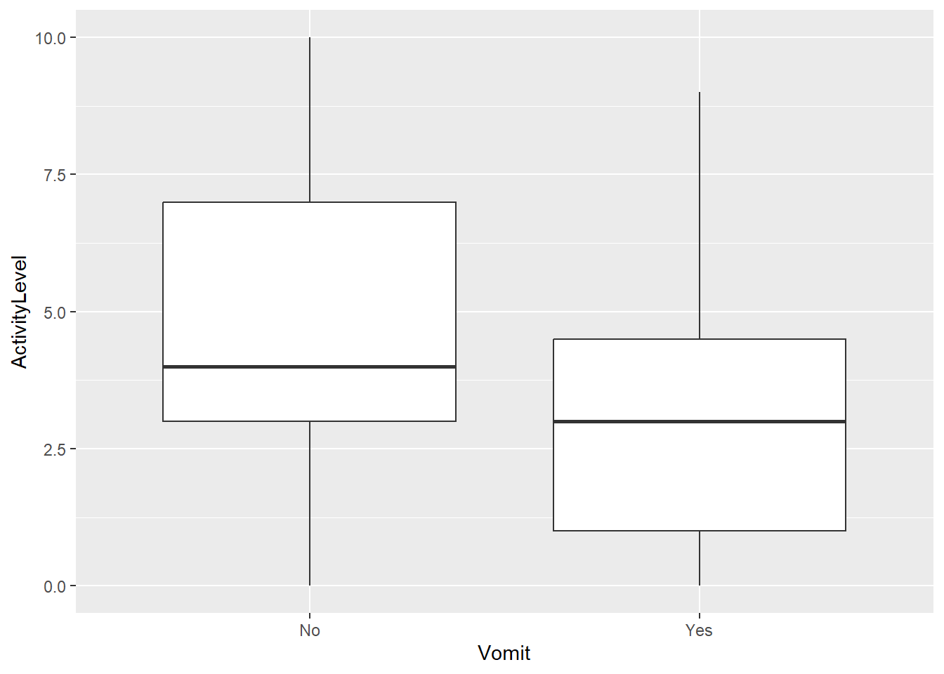
p2 <- dat_sc |> ggplot(aes(x=Vomit,y=ActivityLevel)) + geom_boxplot()
plot(p2)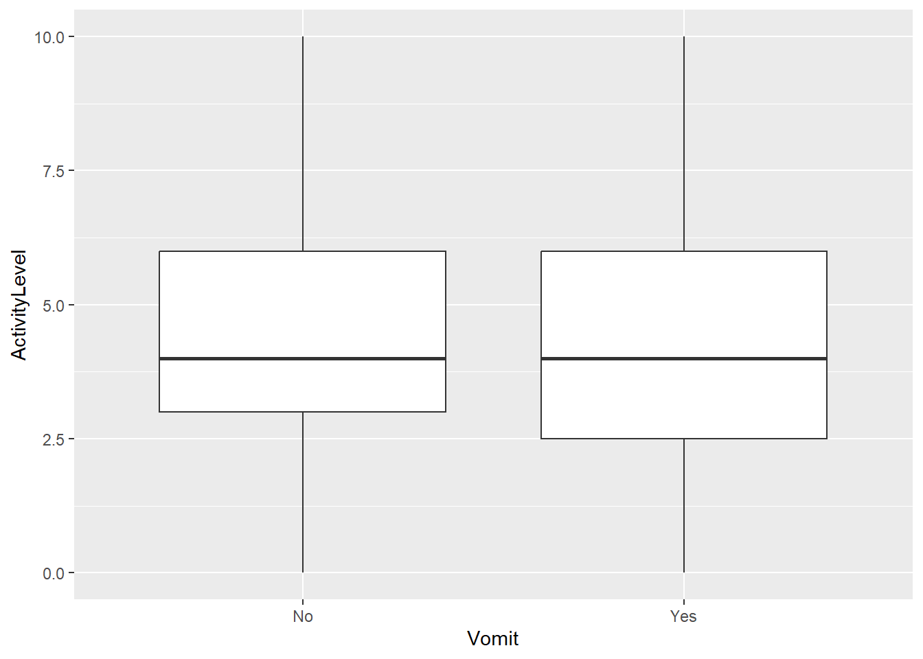
That means any statistical conclusions based on the scrambled data are not valid. This kind of data is just useful at testing the overall workflow and making sure everything can run, but one can’t conclude anything from it.
It is of course possible to try to scramble while preserving potential correlations, but that gets tricky and at this stage one might maybe just re-create the data based on some of the concepts discussed in the previous unit.
Summary
Scrambling the original data is generally fairly easy. It can be useful to for sharing with others or some AI system with reduced issues of confidentiality. One can use it to test if the whole analysis workflow runs. However, one cannot test methods since one doesn’t know what patterns the models should detect, and any statistical conclusions based on the scrambled data are not very meaningful.
Further Resources
The synthpop R package might be useful. It doesn’t quite preserve the original data, it’s more similar to the approach discussed in the unit Generating synthetic data based on existing data. But you can get data that is very close to the original, thus might often give you what you wanted to get when you considered the scrambling approach.