# make sure the packages are installed
# Load required packages
library(dplyr)
library(purrr)
library(lubridate)
library(ggplot2)Generating synthetic data with R
Overview
In this unit, we look at a few examples of generating synthetic data with R.
Learning Objectives
- Be able to generate synthetic data with
Rcode.
Introduction
While there are R packages available that help with the generation of synthetic data - and we will discuss them in a different unit, it is also fairly easy to use basic R functionality to generate simulated data. We’ll do a few examples to show how this can be done.
AI tools are very useful for generating synthetic data. In fact, the code in the examples below was partially generated through back and forth with ChatGPT, together with some manual editing.
Example 1
For the first example, we’ll generate a simple dataset of some hypothetical clinical trial for some treatment (say, a Cholesterol lowering medication) and its impact on outcomes such as Cholesterol levels and adverse events.
It is often useful to go slow and type your own code, or copy and paste the code chunks below and execute one at a time. Note that typing out the code yourself rather than pasting can help improve your muscle memory and retention of what you’re doing! However, if you are in a hurry, you can find the code for this example in this file.
In the code below, you might be wondering what the dplyr::glimpse() and similar such notation is about. This notation indicates explicitly from which package the function comes. Once you loaded a package, that’s not necessary anymore, just using glimpse() would work equally. But it is often nice to quickly see what package a function comes from. An important thing to note is that some packages share function names. In such cases, if a function appears in multiple packages in your environment, R will default to using the one from the most recently loaded package. Using explicit notation is a good way to be sure you’re using the function you want! Thus, you’ll see me use the explicit notation often, though not always. It’s typically a matter of being more explicit versus typing less. I switch back and forth.
Setup
We’ll start by loading the packages used in the code below. While we will not use packages that are specifically meant to generate synthetic data, we will still use several common packages that make data generation tasks easier. That said, you could also do all of this with base R and no additional packages.
# Set a seed for reproducibility
set.seed(123)
# Define the number of observations (patients) to generate
n_patients <- 100
Generating data
# Create an empty data frame with placeholders for variables
syn_dat <- data.frame(
  PatientID = numeric(n_patients),
  Age = numeric(n_patients),
  Gender = character(n_patients),
  TreatmentGroup = character(n_patients),
  EnrollmentDate = lubridate::as_date(character(n_patients)),
  BloodPressure = numeric(n_patients),
  Cholesterol = numeric(n_patients),
  AdverseEvent = integer(n_patients)
)

# Variable 1: Patient ID
syn_dat$PatientID <- 1:n_patients

# Variable 2: Age (numeric variable)
syn_dat$Age <- round(rnorm(n_patients, mean = 45, sd = 10), 1)

# Variable 3: Gender (categorical variable)
syn_dat$Gender <- purrr::map_chr(sample(c("Male", "Female"), n_patients, replace = TRUE), as.character)

# Variable 4: Treatment Group (categorical variable)
syn_dat$TreatmentGroup <- purrr::map_chr(sample(c("A", "B", "Placebo"), n_patients, replace = TRUE), as.character)

# Variable 5: Date of Enrollment (date variable)
syn_dat$EnrollmentDate <- lubridate::as_date(sample(seq(from = lubridate::as_date("2022-01-01"), to = lubridate::as_date("2022-12-31"), by = "days"), n_patients, replace = TRUE))

# Variable 6: Blood Pressure (numeric variable)
syn_dat$BloodPressure <- round(runif(n_patients, min = 90, max = 160), 1)

# Variable 7: Cholesterol Level (numeric variable)
# Option 1: Cholesterol is independent of treatment
#syn_dat$Cholesterol <- round(rnorm(n_patients, mean = 200, sd = 30), 1)

# Option 2: Cholesterol is dependent on treatment
syn_dat$Cholesterol[syn_dat$TreatmentGroup == "A"] <- round(rnorm(sum(syn_dat$TreatmentGroup == "A"), mean = 160, sd = 10), 1)
syn_dat$Cholesterol[syn_dat$TreatmentGroup == "B"] <- round(rnorm(sum(syn_dat$TreatmentGroup == "B"), mean = 180, sd = 10), 1)
syn_dat$Cholesterol[syn_dat$TreatmentGroup == "Placebo"] <- round(rnorm(sum(syn_dat$TreatmentGroup == "Placebo"), mean = 200, sd = 10), 1)

# Variable 8: Adverse Event (binary variable, 0 = No, 1 = Yes)
# Option 1: Adverse events are independent of treatment
#syn_dat$AdverseEvent <- purrr::map_int(sample(0:1, n_patients, replace = TRUE, prob = c(0.8, 0.2)), as.integer)

# Option 2: Adverse events are influenced by treatment status
syn_dat$AdverseEvent[syn_dat$TreatmentGroup == "A"] <- purrr::map_int(sample(0:1, sum(syn_dat$TreatmentGroup == "A"), replace = TRUE, prob = c(0.5, 0.5)), as.integer)
syn_dat$AdverseEvent[syn_dat$TreatmentGroup == "B"] <- purrr::map_int(sample(0:1, sum(syn_dat$TreatmentGroup == "B"), replace = TRUE, prob = c(0.7, 0.3)), as.integer)
syn_dat$AdverseEvent[syn_dat$TreatmentGroup == "Placebo"] <- purrr::map_int(sample(0:1, sum(syn_dat$TreatmentGroup == "Placebo"), replace = TRUE, prob = c(0.9, 0.1)), as.integer)


# Print the first few rows of the generated data
head(syn_dat)
PatientID Age Gender TreatmentGroup EnrollmentDate BloodPressure Cholesterol
1 1 39.4 Female B 2022-08-25 152.0 179.7
2 2 42.7 Female B 2022-06-14 128.7 192.2
3 3 60.6 Female A 2022-04-17 153.4 150.6
4 4 45.7 Male B 2022-02-02 131.1 171.7
5 5 46.3 Female A 2022-03-24 119.6 160.5
6 6 62.2 Female A 2022-12-20 156.5 154.3
AdverseEvent
1 1
2 0
3 0
4 0
5 1
6 1# Save the simulated data to a CSV and Rds file
write.csv(syn_dat, "syn_dat.csv", row.names = FALSE)
# if we wanted an RDS version
#saveRDS(syn_dat, here("data","syn_dat.Rds"))Checking data
Take a peek at the generated data.
summary(syn_dat) PatientID Age Gender TreatmentGroup
Min. : 1.00 Min. :21.90 Length:100 Length:100
1st Qu.: 25.75 1st Qu.:40.08 Class :character Class :character
Median : 50.50 Median :45.60 Mode :character Mode :character
Mean : 50.50 Mean :45.90
3rd Qu.: 75.25 3rd Qu.:51.92
Max. :100.00 Max. :66.90
EnrollmentDate BloodPressure Cholesterol AdverseEvent
Min. :2022-01-08 Min. : 91.3 Min. :129.6 Min. :0.00
1st Qu.:2022-04-06 1st Qu.:110.7 1st Qu.:160.7 1st Qu.:0.00
Median :2022-06-25 Median :130.8 Median :176.3 Median :0.00
Mean :2022-06-30 Mean :128.0 Mean :175.2 Mean :0.29
3rd Qu.:2022-10-04 3rd Qu.:147.4 3rd Qu.:188.7 3rd Qu.:1.00
Max. :2022-12-30 Max. :159.5 Max. :223.7 Max. :1.00 dplyr::glimpse(syn_dat) Rows: 100
Columns: 8
$ PatientID <int> 1, 2, 3, 4, 5, 6, 7, 8, 9, 10, 11, 12, 13, 14, 15, 16, …
$ Age <dbl> 39.4, 42.7, 60.6, 45.7, 46.3, 62.2, 49.6, 32.3, 38.1, 4…
$ Gender <chr> "Female", "Female", "Female", "Male", "Female", "Female…
$ TreatmentGroup <chr> "B", "B", "A", "B", "A", "A", "B", "Placebo", "A", "Pla…
$ EnrollmentDate <date> 2022-08-25, 2022-06-14, 2022-04-17, 2022-02-02, 2022-0…
$ BloodPressure <dbl> 152.0, 128.7, 153.4, 131.1, 119.6, 156.5, 139.6, 118.9,…
$ Cholesterol <dbl> 179.7, 192.2, 150.6, 171.7, 160.5, 154.3, 172.8, 189.2,…
$ AdverseEvent <int> 1, 0, 0, 0, 1, 1, 1, 0, 0, 0, 0, 0, 0, 0, 0, 0, 0, 0, 1…# Frequency table for adverse events stratified by treatment
table(syn_dat$AdverseEvent,syn_dat$TreatmentGroup)
     A  B Placebo
  0 28 19      24
  1 15 11       3
# ggplot2 boxplot for cholesterol by treatment group
ggplot(syn_dat, aes(x = TreatmentGroup, y = Cholesterol)) +
geom_boxplot() +
labs(x = "Treatment Group", y = "Cholesterol Level") +
theme_bw()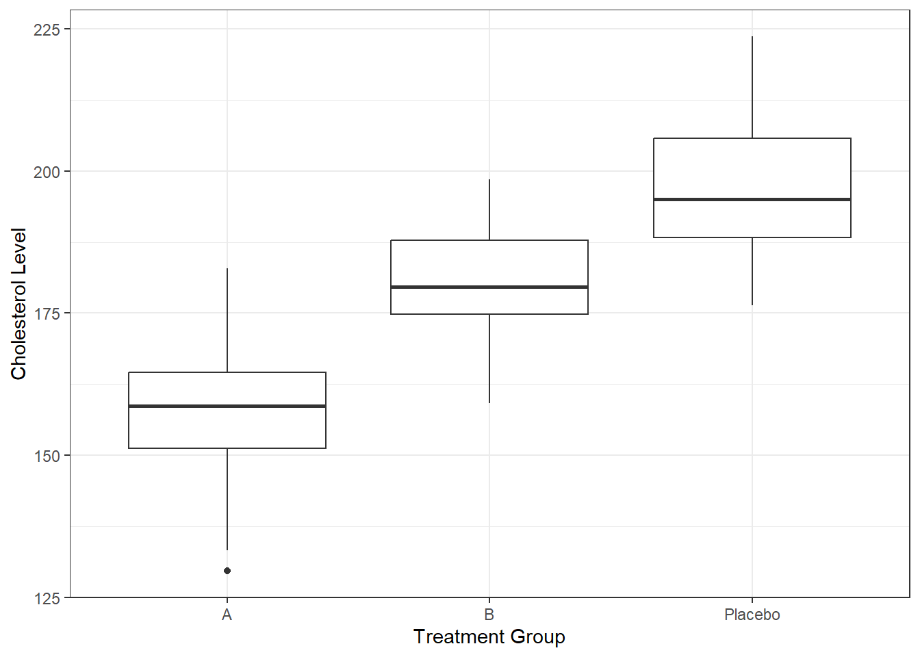
This concludes our first example. This was a very simple setup, with rectangular data. You often encounter these kind of data in clinical trials. As you generate your data, you can build in any dependencies between variables you want to explore. Then later, when you use the data to test your analysis code, you can see if your analysis code can detect the dependencies you built in. We’ll come back to that.
You could also add further complexities into your synthetic data, for instance you could set some values to be missing, or you could add some outliers. The goal is to generate data that has as the important features of your real dataset to allow you to test your analysis approach on data where you now the truth (since you generated it). If your analysis works on your generated data, there is hope it might also work on the real data (for which of course you don’t know the truth). We’ll define in a later unit what we mean by “your analysis works”. But basically, you want to be able to recover the patterns/dependencies you built into your data with your analysis methods.
Example 2
In this example, we’ll generate a dataset that has a more complex structure. We’ll generate a dataset that has a longitudinal structure, i.e. repeated measurements over time. We’ll also generate a dataset that has a hierarchical structure, i.e. measurements nested within groups.
We’ll walk slowly through the code chunks, you can find all the code in this file.
Setup
The usual setup steps.
# make sure the packages are installed
# Load required packages
library(dplyr)
library(ggplot2)
library(here)
# Set seed for reproducibility
set.seed(123)
# Number of patients in each treatment group
num_patients <- 20
# Number of days and samples per patient
num_days <- 7
num_samples_per_day <- 1Generating data
# Treatment group levels
treatment_groups <- c("Low Dose", "High Dose")

# Generate patient IDs
patient_ids <- rep(1:num_patients, each = num_days)

# Generate treatment group assignments for each patient
treatment_assignments <- rep(sample(treatment_groups, num_patients, replace = TRUE),
                             each = num_days)

# Generate day IDs for each patient
day_ids <- rep(1:num_days, times = num_patients)

# Function to generate drug concentrations with variability
generate_drug_concentrations <- function(day, dose_group, patient_id) {
  baseline_concentration <- ifelse(dose_group == "Low Dose", 8, 15)
  patient_variation <- rnorm(1, mean = 0, sd = 1)
  time_variation <- exp(-0.1*day)
  baseline_concentration * time_variation + patient_variation
}


# Generate drug concentrations for each sample
drug_concentrations <- mapply(generate_drug_concentrations,
                              day = rep(day_ids, each = num_samples_per_day),
                              dose_group = treatment_assignments,
                              patient_id = rep(1:num_patients, each = num_days))


# Flatten the matrix to a vector
drug_concentrations <- as.vector(drug_concentrations)

# Generate cholesterol levels for each sample
# (assuming a positive correlation with drug concentration)
cholesterol_levels <- drug_concentrations +
  rnorm(num_patients * num_days * num_samples_per_day, mean = 0, sd = 5)

# Generate adverse events based on drug concentration
# (assuming a higher chance of adverse events with higher concentration)
# Sigmoid function to map concentrations to probabilities
adverse_events_prob <- plogis(drug_concentrations / 10)
adverse_events <- rbinom(num_patients * num_days * num_samples_per_day,
                         size = 1, prob = adverse_events_prob)

# Create a data frame
syn_dat2 <- data.frame(
  PatientID = rep(patient_ids, each = num_samples_per_day),
  TreatmentGroup = rep(treatment_assignments, each = num_samples_per_day),
  Day = rep(day_ids, each = num_samples_per_day),
  DrugConcentration = drug_concentrations,
  CholesterolLevel = cholesterol_levels,
  AdverseEvent = adverse_events
)
Checking data
Take a peek at the generated data.
# Print the first few rows of the generated dataset
print(head(syn_dat2))
PatientID TreatmentGroup Day DrugConcentration CholesterolLevel AdverseEvent
1 1 Low Dose 1 8.462781 12.401475 0
2 1 Low Dose 2 6.909660 10.754871 0
3 1 Low Dose 3 6.327317 7.988330 0
4 1 Low Dose 4 5.473243 0.431360 1
5 1 Low Dose 5 4.296404 3.699141 0
6 1 Low Dose 6 6.177406 4.775430 1summary(syn_dat2) PatientID TreatmentGroup Day DrugConcentration
Min. : 1.00 Length:140 Min. :1 Min. : 2.081
1st Qu.: 5.75 Class :character 1st Qu.:2 1st Qu.: 5.174
Median :10.50 Mode :character Median :4 Median : 7.056
Mean :10.50 Mean :4 Mean : 7.593
3rd Qu.:15.25 3rd Qu.:6 3rd Qu.: 9.738
Max. :20.00 Max. :7 Max. :14.933
CholesterolLevel AdverseEvent
Min. :-4.494 Min. :0.0000
1st Qu.: 3.844 1st Qu.:0.0000
Median : 7.234 Median :1.0000
Mean : 7.855 Mean :0.6571
3rd Qu.:11.259 3rd Qu.:1.0000
Max. :24.422 Max. :1.0000 dplyr::glimpse(syn_dat2) Rows: 140
Columns: 6
$ PatientID <int> 1, 1, 1, 1, 1, 1, 1, 2, 2, 2, 2, 2, 2, 2, 3, 3, 3, 3…
$ TreatmentGroup <chr> "Low Dose", "Low Dose", "Low Dose", "Low Dose", "Low…
$ Day <int> 1, 2, 3, 4, 5, 6, 7, 1, 2, 3, 4, 5, 6, 7, 1, 2, 3, 4…
$ DrugConcentration <dbl> 8.462781, 6.909660, 6.327317, 5.473243, 4.296404, 6.…
$ CholesterolLevel <dbl> 12.4014754, 10.7548711, 7.9883301, 0.4313600, 3.6991…
$ AdverseEvent <int> 0, 0, 0, 1, 0, 1, 1, 0, 0, 1, 1, 1, 0, 1, 1, 0, 1, 1…Exploratory plot
# Plot drug concentrations over time for each individual using ggplot2
p1 <- ggplot(syn_dat2, aes(x = Day, y = DrugConcentration,
                      group = as.factor(PatientID), color = TreatmentGroup)) +
  geom_line() +
  labs(title = "Drug Concentrations Over Time",
       x = "Day",
       y = "Drug Concentration",
       color = "TreatmentGroup") +
  theme_minimal()
plot(p1)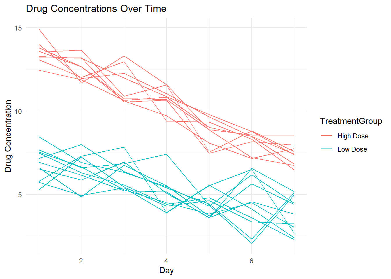
p2 <- ggplot(syn_dat2, aes(x = as.factor(AdverseEvent), y = DrugConcentration,
                           fill = TreatmentGroup)) +
  geom_boxplot(width = 0.7, position = position_dodge(width = 0.8), color = "black") +
  geom_point(aes(color = TreatmentGroup), position = position_dodge(width = 0.8),
             size = 3, shape = 16) +  # Overlay raw data points
  labs(
    x = "Adverse Events",
    y = "Drug Concentration",
    title = "Boxplot of Drug Concentration by Adverse Events and Treatment"
  ) +
  scale_color_manual(values = c("A" = "blue", "B" = "red")) +  # Customize color for each treatment
  theme_minimal() +
  theme(legend.position = "top")
plot(p2)
Warning: No shared levels found between `names(values)` of the manual scale and the
data's colour values.
No shared levels found between `names(values)` of the manual scale and the
data's colour values.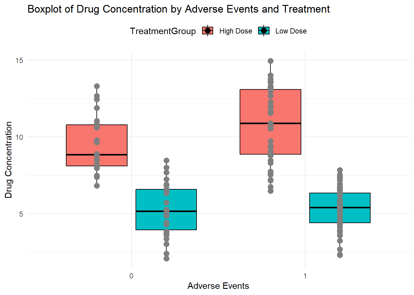
This dataset has a bit more complicated structure than the previous one, but it isn’t much harder to generate it with code. You’ll want to generate your data such that it mimics the real data you plan on analyzing.
Save data
# Save the simulated data to a CSV or Rds file
write.csv(syn_dat2, "syn_dat2.csv", row.names = FALSE)
# if we wanted an RDS version
#saveRDS(syn_dat2, here("data","syn_dat2.Rds"))
We are saving the data as CSV and Rds files. CSV files are readable with pretty much any software and thus very portable. Rds files are R-specific, thus not as flexible. The advantage of Rds files is that they are generally smaller, and they retain information about the variables, e.g. if they are factor or numeric variables. Either format works, sometimes one or the other might be better.
Summary
It is fairly easy to generate synthetic data with some basic R commands, and it’s even easier if you use some LLM AI tool to help you write the code.
Since you generate the data, you can decide what dependencies between variables you want to add, and you can then test your models to see if they can find those patterns. We’ll get to that in another unit.
Further Resources
While the manual generation of data is generally fairly easy and gives you the most control, sometimes using R packages specifically designed for this purpose can be useful. We’ll look at a few in a later unit.