# Load the readr package for reading csv data
library(readr)
library(dplyr)
library(broom)
library(parsnip)
library(here)

# Read in the csv data
data <- read_csv("syn_dat.csv")Use synthetic data to test models
Overview
In this unit, we explore the use of synthetic data to test your models.
Learning Objectives
- Understand the use of synthetic data for testing models.
- Be able to implement model testing on synthetic data in R.
Introduction
At the beginning of this module, I mentioned that one great use-case of synthetic data is the ability to see if whatever patterns you stuck into the data when you generated it can be recovered by your analysis. If your analysis fails to recover what you built, it means your model is likely not suitable and you need to modify it.
Of course, keep in mind that just because your model can recover the patterns/correlations you stuck into the data doesn’t mean it can do the same for the real data, or that any patterns in the real data are the same. However, if you can NOT recover the patterns for your simulated data, it’s a strong sign to stop and reconsider your analysis approach. It will very likely also not produce useful results for the real data (but you won’t know, since you don’t know what processes generated the real data).
An example
We will revisit the first example from the Generating synthetic data with R unit. If you don’t remember, take a look at the code shown in that unit to see that we created a variable called BloodPressure which was randomly distributed, and a variable called Cholesterol which varied by treatment group.
If we fit a model, we expect to recover these patterns. We can for instance fit a linear model with Cholesterol as the outcome and BloodPressure and TreatmentGroup as predictors.
Here’s code to do that (you can again find the full R script here).
Setting things up
We’ll do a little bit of processing before fitting
# select variables of interest
# not strictly needed, but can sometimes make for more robust code to only keep what's necessary
data <- data %>%
  select(Cholesterol, BloodPressure, TreatmentGroup)

# Standardize BloodPressure and Cholesterol
# Helps with interpretation of coefficients
data <- data %>%
  mutate(
    BloodPressure = scale(BloodPressure),
    Cholesterol = scale(Cholesterol)
  )
# turn TreatmentGroup into a factor
data$TreatmentGroup <- as.factor(data$TreatmentGroup)

# check to make sure data looks ok before fitting
summary(data)
Cholesterol.V1 BloodPressure.V1 TreatmentGroup
Min. :-2.38863692699e+00 Min. :-1.72011727192e+00 A :43
1st Qu.:-7.63161855038e-01 1st Qu.:-8.10951978975e-01 B :30
Median : 5.87369736145e-02 Median : 1.35753042193e-01 Placebo:27
Mean :-6.00000000000e-16 Mean : 3.00000000000e-16
3rd Qu.: 7.05262485325e-01 3rd Qu.: 9.11183053336e-01
Max. : 2.53752102054e+00 Max. : 1.48014455924e+00 Fitting the first model
# Fit linear model
model1 <- linear_reg() %>%
  set_engine("lm") %>%
  parsnip::fit(Cholesterol ~ BloodPressure + TreatmentGroup, data = data)
tidy(model1)
# A tibble: 4 × 5
term estimate std.error statistic p.value
<chr> <dbl> <dbl> <dbl> <dbl>
1 (Intercept) -0.898 0.0822 -10.9 1.58e-18
2 BloodPressure -0.0822 0.0548 -1.50 1.37e- 1
3 TreatmentGroupB 1.19 0.129 9.24 6.48e-15
4 TreatmentGroupPlacebo 2.00 0.133 15.1 4.05e-27glance(model1)# A tibble: 1 × 12
r.squared adj.r.squared sigma statistic p.value df logLik AIC BIC
<dbl> <dbl> <dbl> <dbl> <dbl> <dbl> <dbl> <dbl> <dbl>
1 0.718 0.709 0.539 81.6 2.61e-26 3 -78.0 166. 179.
# ℹ 3 more variables: deviance <dbl>, df.residual <int>, nobs <int>We find what we hope to find. The blood pressure variable shows no noticeable correlation with cholesterol, while treatment group does.
We can explore other models. Here is one with an interaction term between BloodPressure and TreatmentGroup. We know there is none, since we know how the data was generated. So to test our model, we fit it to confirm that this is what we get:
# fit a model with interaction
model2 <- linear_reg() %>%
  set_engine("lm") %>%
  parsnip::fit(Cholesterol ~ BloodPressure + TreatmentGroup + BloodPressure*TreatmentGroup , data = data)
tidy(model2)
# A tibble: 6 × 5
term estimate std.error statistic p.value
<chr> <dbl> <dbl> <dbl> <dbl>
1 (Intercept) -0.901 0.0825 -10.9 2.15e-18
2 BloodPressure -0.139 0.0766 -1.82 7.18e- 2
3 TreatmentGroupB 1.19 0.131 9.10 1.52e-14
4 TreatmentGroupPlacebo 2.02 0.134 15.1 8.90e-27
5 BloodPressure:TreatmentGroupB 0.0856 0.129 0.665 5.08e- 1
6 BloodPressure:TreatmentGroupPlacebo 0.163 0.144 1.13 2.60e- 1glance(model2)# A tibble: 1 × 12
r.squared adj.r.squared sigma statistic p.value df logLik AIC BIC
<dbl> <dbl> <dbl> <dbl> <dbl> <dbl> <dbl> <dbl> <dbl>
1 0.722 0.708 0.541 48.9 1.09e-24 5 -77.3 169. 187.
# ℹ 3 more variables: deviance <dbl>, df.residual <int>, nobs <int>And we do see no evidence for interaction being present. So for this simple example, the model works, namely it recovers the patterns we stuck into the data. This means it might be ok to use this model on our real data.
Let’s now look at an example where the model does not properly recover the pattern in the data.
A failing example
We’ll start with the same data as before, but now mess around with it. Specifically, I’m creating a new variable called Drug and a new cholesterol variable that depends on drug concentration in a nonlinear manner.
# Load the readr package for reading csv data
library(readr)
library(dplyr)
library(here)
library(tidymodels)
library(vip)

# Read in the csv data
set.seed(123)
data <- read_csv("syn_dat.csv")
# Make Cholesterol depend on blood pressure in a nonlinear manner
data$Drug <- runif(nrow(data),min = 100, max = 200)
# making up Cholesterol value as function of Drug
# this equation makes it such that cholesterol depends on drug in a nonlinear manner
data$Cholesterol2 <- sqrt(100^2 + 10* (mean(data$Drug) - data$Drug)^2)
# plotting correlation between Drug and new cholesterol variables
ggplot(data,aes(x=Drug, y=Cholesterol2)) + geom_point()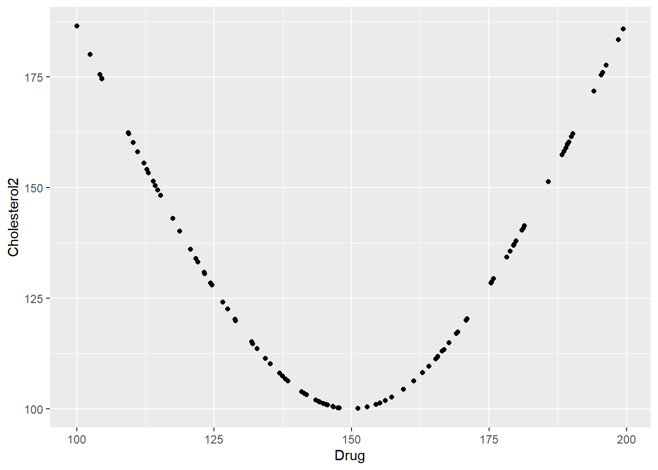
# select variables of interest
# not strictly needed, but can sometimes make for more robust code to only keep what's necessary
data <- data %>%
  select(Cholesterol2, Drug, BloodPressure, TreatmentGroup)

# Standardize continuous variables
# Helps with interpretation of coefficients
data <- data %>%
  mutate(
    BloodPressure = scale(BloodPressure),
    Drug = scale(Drug),
    Cholesterol2 = scale(Cholesterol2)
  )
# turn TreatmentGroup into a factor
data$TreatmentGroup <- as.factor(data$TreatmentGroup)

# check to make sure data looks ok before fitting
summary(data)
Cholesterol2.V1 Drug.V1
Min. :-1.22222514059e+00 Min. :-1.747166617720
1st Qu.:-9.20323907468e-01 1st Qu.:-0.888043951821
Median :-1.25708288800e-01 Median :-0.112943096895
Mean : 1.00000000000e-16 Mean : 0.000000000000
3rd Qu.: 8.74199838460e-01 3rd Qu.: 0.901461486215
Max. : 2.10805990267e+00 Max. : 1.739364949530
BloodPressure.V1 TreatmentGroup
Min. :-1.72011727192e+00 A :43
1st Qu.:-8.10951978975e-01 B :30
Median : 1.35753042193e-01 Placebo:27
Mean : 3.00000000000e-16
3rd Qu.: 9.11183053336e-01
Max. : 1.48014455924e+00 Now we’ll fit another linear model, as before. There is a correlation between dose and cholesterol. But it’s not linear, and therefore the model doesn’t detect it.
# Fit linear model
model1 <- linear_reg() %>%
  set_engine("lm") %>%
  parsnip::fit(Cholesterol2 ~ Drug + BloodPressure + TreatmentGroup, data = data)
broom::tidy(model1)
# A tibble: 5 × 5
term estimate std.error statistic p.value
<chr> <dbl> <dbl> <dbl> <dbl>
1 (Intercept) 0.101 0.155 0.653 0.515
2 Drug 0.0353 0.103 0.343 0.732
3 BloodPressure 0.0574 0.103 0.557 0.579
4 TreatmentGroupB -0.247 0.243 -1.02 0.311
5 TreatmentGroupPlacebo -0.0997 0.251 -0.398 0.692broom::glance(model1)# A tibble: 1 × 12
r.squared adj.r.squared sigma statistic p.value df logLik AIC BIC
<dbl> <dbl> <dbl> <dbl> <dbl> <dbl> <dbl> <dbl> <dbl>
1 0.0142 -0.0273 1.01 0.343 0.848 4 -141. 293. 309.
# ℹ 3 more variables: deviance <dbl>, df.residual <int>, nobs <int>It is always possible to try a more complex model to see if there might be patterns that a linear or other simple model can’t detect. Here, we are trying a random forest model, which can detect more complicated correlations between predictor variables and output. Random forest models don’t produce the standard p-values, but one can look at something called variable importance to see which variables most impact the outcome. And we see that it correctly identifies drug as the most important variable. The other two should really be at zero importance, since they are not correlated with the outcome. But this model is flexible enough to fit to possibly spurious patterns.
# fit a random forest model
# use the workflow approach from tidymodels
rf_mod <- rand_forest(mode = "regression") %>%
  set_engine("ranger", importance = "impurity")
# the recipe, i.e., the model to fit
rf_recipe <-
  recipe(Cholesterol2 ~ Drug + BloodPressure + TreatmentGroup, data = data)

# set up the workflow
rf_workflow <-
  workflow() %>%
  add_model(rf_mod) %>%
  add_recipe(rf_recipe)

# run the fit
model2 <- rf_workflow %>%
      fit(data)

# get variable importance
imp <- model2 %>%
  extract_fit_parsnip() %>%
  vip()
print(imp)
The take-home message from this is that our simulated data showed us that a linear model can’t pick up the pattern, and we need a different model.
Summary
Model testing is one of the most important applications for synthetic data. Since you generated the data and know everything about it, you know exactly what the analysis of the data should find. If your models can’t find the right patterns, it means you need to modify your analysis.