# make sure the packages are installed
# Load required packages
library(here)
library(dplyr)
library(ggplot2)
library(skimr)
library(gtsummary)Generating synthetic data based on existing data
Overview
In this unit, we discuss how to generate synthetic data based on existing data.
Goals
- Be able to generate synthetic data with
Rbased on existing data.
Introduction
You generally want to produce synthetic data that resembles the real data you are interested in. The simplest approach is to just look at the variables of interest in your actual data, then write code to generate synthetic data with those variables and values for each variable that are similar to the original data.
That’s quick, you can use AI to help, and often that’s good enough. But sometimes you might want to generate synthetic data that resembles the original data very closely.
In that case, you will first want to determine the ranges and distributions of your existing data and then use that information to generate new synthetic data.
Essentially, what you want to do is perform descriptive and explorary analysis on your real data, then use what you found to inform the creation of your synthetic data.
AI help
You probably don’t want to feed your real data to the AI. So the first part of summarizing existing data has to be done in a safe/secure space. Once you have good data summaries, you can use AI to generate synthetic data and code.
Example
We’ll use the data we generated in example 1 of the previous tutorial and now assume that this is “real” data and that we want to generate synthetic data that’s similar to the real data.
Setup
First, we do the usual setup steps of package loading and other housekeeping steps.
# Set a seed for reproducibility
set.seed(123)
# Define the number of observations (patients) to generate
n_patients <- 100
Load and explore data
In a first step, we want to understand how each variable in the real data set is distributed, so we can create synthetic data that looks very similar.
We can use various helper functions from different packages to get good descriptive summaries of the data and variables. This code below shows two such helper functions.
Note that we added more information to the table output. The table summary function treats the date variable and patient ID variable as numeric, so the output is somewhat nonsensical. But this is just for internal “quick and dirty” use, so we don’t need to make things pretty. Of course you could if you needed/wanted.
dat <- readRDS("syn_dat.rds")
skimr::skim(dat)| Name | dat |
| Number of rows | 100 |
| Number of columns | 8 |
| _______________________ | |
| Column type frequency: | |
| character | 2 |
| Date | 1 |
| numeric | 5 |
| ________________________ | |
| Group variables | None |
Variable type: character
| skim_variable | n_missing | complete_rate | min | max | empty | n_unique | whitespace |
|---|---|---|---|---|---|---|---|
| Gender | 0 | 1 | 4 | 6 | 0 | 2 | 0 |
| TreatmentGroup | 0 | 1 | 1 | 7 | 0 | 3 | 0 |
Variable type: Date
| skim_variable | n_missing | complete_rate | min | max | median | n_unique |
|---|---|---|---|---|---|---|
| EnrollmentDate | 0 | 1 | 2022-01-08 | 2022-12-30 | 2022-06-25 | 86 |
Variable type: numeric
| skim_variable | n_missing | complete_rate | mean | sd | p0 | p25 | p50 | p75 | p100 | hist |
|---|---|---|---|---|---|---|---|---|---|---|
| PatientID | 0 | 1 | 50.50 | 29.01 | 1.0 | 25.75 | 50.50 | 75.25 | 100.0 | ▇▇▇▇▇ |
| Age | 0 | 1 | 45.90 | 9.14 | 21.9 | 40.08 | 45.60 | 51.92 | 66.9 | ▁▃▇▅▂ |
| BloodPressure | 0 | 1 | 127.96 | 21.31 | 91.3 | 110.67 | 130.85 | 147.38 | 159.5 | ▅▅▅▅▇ |
| Cholesterol | 0 | 1 | 174.67 | 32.58 | 88.9 | 153.23 | 171.85 | 196.62 | 271.0 | ▁▆▇▃▁ |
| AdverseEvent | 0 | 1 | 0.29 | 0.46 | 0.0 | 0.00 | 0.00 | 1.00 | 1.0 | ▇▁▁▁▃ |
gtsummary::tbl_summary(dat, statistic = list(
  all_continuous() ~ "{mean}/{median}/{min}/{max}/{sd}",
  all_categorical() ~ "{n} / {N} ({p}%)"
),)| Characteristic | N = 1001 |
|---|---|
| PatientID | 51/51/1/100/29 |
| Age | 46/46/22/67/9 |
| Gender | |
| Female | 49 / 100 (49%) |
| Male | 51 / 100 (51%) |
| TreatmentGroup | |
| A | 43 / 100 (43%) |
| B | 30 / 100 (30%) |
| Placebo | 27 / 100 (27%) |
| EnrollmentDate | 2022-06-30/2022-06-25/2022-01-08/2022-12-30/107.06744593852 |
| BloodPressure | 128/131/91/160/21 |
| Cholesterol | 175/172/89/271/33 |
| AdverseEvent | 29 / 100 (29%) |
| 1 Mean/Median/Min/Max/SD; n / N (%) | |
We can also look at the distribution of the different variables individually, using e.g., base R commands (or any other package of your choice).
# using base R to explore variable distributions
table(dat$Gender)
Female   Male
49 51 table(dat$TreatmentGroup)
      A       B Placebo
43 30 27 table(dat$AdverseEvent)
 0  1
71 29 hist(dat$Age)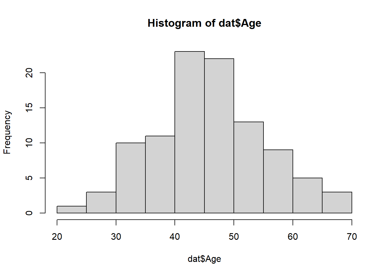
hist(dat$BloodPressure)
hist(dat$Cholesterol)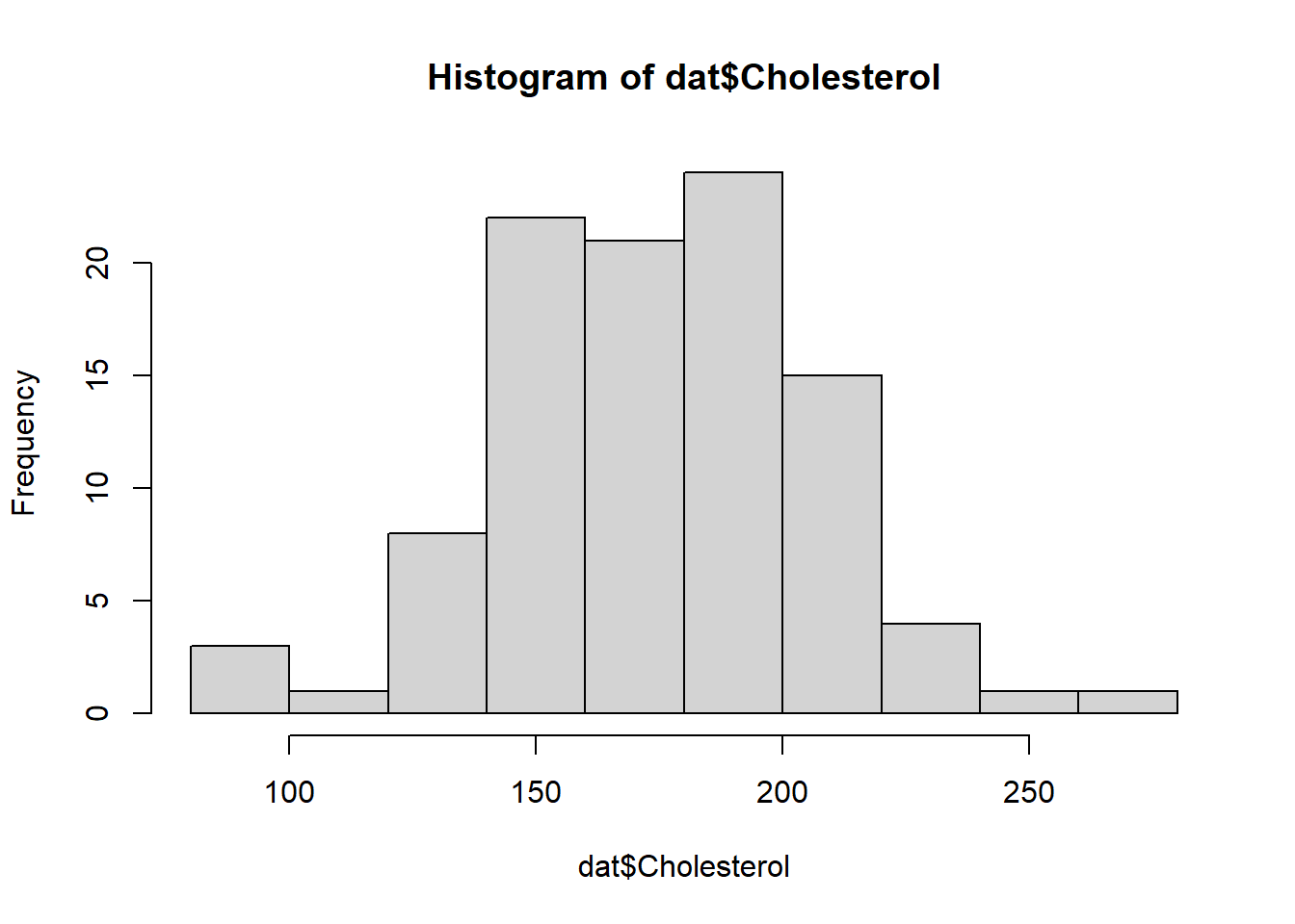
Looks like a normal distribution for age and uniform distribution for blood pressure should work well. That’s of course not surprising since we produced the data that way in an earlier tutorial. But for real data you don’t know what process produced it, you just want to see how things are distributed so you can recreate it that way.
For Cholesterol, the distribution doesn’t look quite normal. That’s because in the original data generating process, we made it dependent on treatment.
If you want to see if there are correlations in the data that you might want to also have in your synthetic data, you can explore those with tables or plots like these.
# explore some correlations between variables
table(dat$AdverseEvent, dat$TreatmentGroup)
     A  B Placebo
  0 28 19      24
1 15 11 3plot(dat$Age, dat$BloodPressure)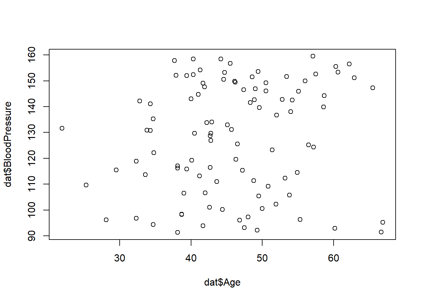
ggplot(dat) + geom_histogram(aes(x = Cholesterol, fill = TreatmentGroup)) `stat_bin()` using `bins = 30`. Pick better value with `binwidth`.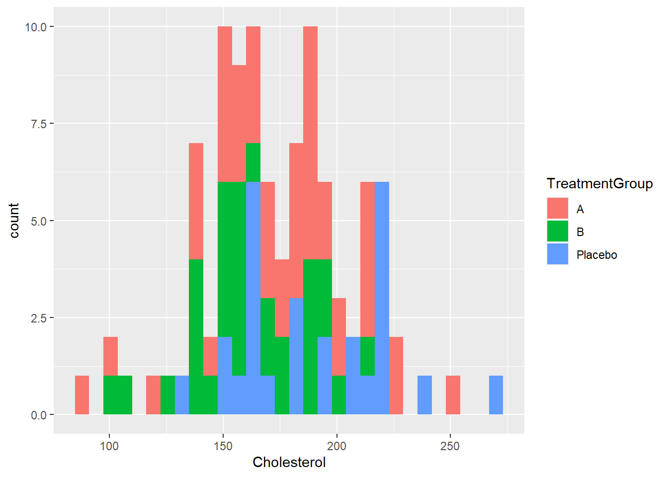
At this stage, it is up to you to decide if you want to try to include correlations between variables that might or might not exist in the real data, or if you just want to give each variable an independent distribution.
Generate data
Now we’ll create synthetic data that is similar to the real data. In this code example, we pull directly from the actual data stored in dat. However, you can also save that information into an intermediary object or file (e.g., save the mean and standard deviation of age) and then just use those summary statistics to generate the synthetic data. This prevents for instance issues with confidentiality if you use AI to help write the synthetic data code.
# Create an empty data frame with placeholders for variables
syn_dat <- data.frame(
  PatientID = numeric(n_patients),
  Age = numeric(n_patients),
  Gender = character(n_patients),
  TreatmentGroup = character(n_patients),
  EnrollmentDate = lubridate::as_date(character(n_patients)),
  BloodPressure = numeric(n_patients),
  Cholesterol = numeric(n_patients),
  AdverseEvent = integer(n_patients)
)

# Variable 1: Patient ID
# can be exactly the same as the original
syn_dat$PatientID <- 1:n_patients

# Variable 2: Age (numeric variable)
# creating normally distributed values with the mean and SD taken
# from the real data
syn_dat$Age <- round(rnorm(n_patients, mean = mean(dat$Age), sd = sd(dat$Age)), 1)

# Variable 3: Gender (categorical variable)
# create with probabilities based on real data distribution
syn_dat$Gender <- sample(c("Male", "Female"),
                         n_patients, replace = TRUE,
                         prob = as.numeric(table(dat$Gender)/100))

# Variable 4: Treatment Group (categorical variable)
# create with probabilities based on real data distribution
syn_dat$TreatmentGroup <- sample(c("A", "B", "Placebo"),
                                 n_patients,
                                 replace = TRUE,
                                 prob = as.numeric(table(dat$TreatmentGroup)/100))

# Variable 5: Date of Enrollment (date variable)
# use same start and end dates as real data
syn_dat$EnrollmentDate <- lubridate::as_date(sample(seq(from = min(dat$EnrollmentDate),
                                                        to = max(dat$EnrollmentDate),
                                                        by = "days"), n_patients, replace = TRUE))

# Variable 6: Blood Pressure (numeric variable)
# use uniform distribution as indicated by histogram of real data
# use same min and max values as real data
syn_dat$BloodPressure <- round(runif(n_patients,
                                     min = min(dat$BloodPressure),
                                     max = max(dat$BloodPressure)), 1)

# Variable 7: Cholesterol Level (numeric variable)
# here, we re-create it based on the overall data distribution pattern
# since the data didn't quite look like a normal distribution,
# here we'll just use it as its own distribution and sample right from the data
# note that this breaks the association with treatment group
# for real data, we wouldn't know if there is any, but if we suspect, we could
# generate data with and without such associations and explore its impact on model performance
syn_dat$Cholesterol <- sample(dat$Cholesterol,
                                    size = n_patients,
                                    replace = TRUE)


# Variable 8: Adverse Event (binary variable, 0 = No, 1 = Yes)
# we implement this variable by taking into account different probabilities stratified by treatment
probA = as.numeric(table(dat$AdverseEvent,dat$TreatmentGroup)[,1])/sum(table(dat$AdverseEvent,dat$TreatmentGroup)[,1])
probB = as.numeric(table(dat$AdverseEvent,dat$TreatmentGroup)[,2])/sum(table(dat$AdverseEvent,dat$TreatmentGroup)[,2])
probP = as.numeric(table(dat$AdverseEvent,dat$TreatmentGroup)[,3])/sum(table(dat$AdverseEvent,dat$TreatmentGroup)[,3])

# this re-creates the correlation we find between those two variables
syn_dat$AdverseEvent[syn_dat$TreatmentGroup == "A"] <- sample(0:1, sum(syn_dat$TreatmentGroup == "A"), replace = TRUE, prob = probA)
syn_dat$AdverseEvent[syn_dat$TreatmentGroup == "B"] <- sample(0:1, sum(syn_dat$TreatmentGroup == "B"), replace = TRUE, prob = probB)
syn_dat$AdverseEvent[syn_dat$TreatmentGroup == "Placebo"] <- sample(0:1, sum(syn_dat$TreatmentGroup == "Placebo"), replace = TRUE, prob = probP)
You can always make your synthetic data partially different from the real data for important quantities (e.g., your main input/exposure or outcome of interest) to explore different implications and model performance.
Check and save data
Quick peek at generated data to make sure things look ok, then we can save it.
# Print the first few rows of the generated data
head(syn_dat)
PatientID Age Gender TreatmentGroup EnrollmentDate BloodPressure Cholesterol
1 1 34.7 Male Placebo 2022-05-02 152.9 218.7
2 2 49.9 Male B 2022-10-12 150.3 140.6
3 3 53.2 Female Placebo 2022-04-11 144.2 186.7
4 4 44.4 Female A 2022-07-28 117.0 205.4
5 5 57.3 Female Placebo 2022-01-23 94.2 140.9
6 6 37.4 Female B 2022-07-23 116.2 160.1
AdverseEvent
1 0
2 1
3 0
4 1
5 0
6 1# quick summaries
summary(syn_dat) PatientID Age Gender TreatmentGroup
Min. : 1.00 Min. :23.10 Length:100 Length:100
1st Qu.: 25.75 1st Qu.:40.65 Class :character Class :character
Median : 50.50 Median :46.20 Mode :character Mode :character
Mean : 50.50 Mean :46.71
3rd Qu.: 75.25 3rd Qu.:51.60
Max. :100.00 Max. :65.50
EnrollmentDate BloodPressure Cholesterol AdverseEvent
Min. :2022-01-15 Min. : 91.6 Min. : 97.6 Min. :0.00
1st Qu.:2022-04-15 1st Qu.:108.9 1st Qu.:158.0 1st Qu.:0.00
Median :2022-07-02 Median :125.0 Median :167.5 Median :0.00
Mean :2022-07-01 Mean :125.0 Mean :175.4 Mean :0.31
3rd Qu.:2022-09-27 3rd Qu.:142.3 3rd Qu.:197.4 3rd Qu.:1.00
Max. :2022-12-26 Max. :159.2 Max. :248.7 Max. :1.00 dplyr::glimpse(syn_dat) Rows: 100
Columns: 8
$ PatientID <int> 1, 2, 3, 4, 5, 6, 7, 8, 9, 10, 11, 12, 13, 14, 15, 16, …
$ Age <dbl> 34.7, 49.9, 53.2, 44.4, 57.3, 37.4, 49.5, 49.6, 37.8, 3…
$ Gender <chr> "Male", "Male", "Female", "Female", "Female", "Female",…
$ TreatmentGroup <chr> "Placebo", "B", "Placebo", "A", "Placebo", "B", "Placeb…
$ EnrollmentDate <date> 2022-05-02, 2022-10-12, 2022-04-11, 2022-07-28, 2022-0…
$ BloodPressure <dbl> 152.9, 150.3, 144.2, 117.0, 94.2, 116.2, 110.0, 149.3, …
$ Cholesterol <dbl> 218.7, 140.6, 186.7, 205.4, 140.9, 160.1, 229.0, 204.7,…
$ AdverseEvent <int> 0, 1, 0, 1, 0, 1, 0, 0, 0, 0, 0, 0, 1, 0, 0, 1, 1, 0, 0…# Frequency table for adverse events stratified by treatment
table(syn_dat$AdverseEvent,syn_dat$TreatmentGroup)
     A  B Placebo
  0 31 15      23
  1 17 12       2
# ggplot2 boxplot for cholesterol by treatment group
ggplot(syn_dat, aes(x = TreatmentGroup, y = Cholesterol)) +
geom_boxplot() +
labs(x = "Treatment Group", y = "Cholesterol Level") +
theme_bw()
# Save the simulated data to a CSV file
write.csv(syn_dat, "syn_dat_new.csv", row.names = FALSE)
Summary
The process of generating synthetic data based on existing data is fairly straightforward:
- Load existing data.
- Look at distributions/frequencies of variables of interest.
- Generate new data with variables that are distributed like original data.
Sometimes, you can just look at your original data and make up new data that’s roughly similar. At other times you want to be very close, in that case you need to either draw new values from distributions that are well-describe the original data, or you need to re-sample the original data (with or without replacement).
Fortunately, most of the time it’s good enough to get your data somewhat similar to the original. You would hope/expect any kind of statistical method to work well on different sets of data that are roughly similar. If that’s not the case, your method might not be very robust and might require changes.
Further Resources
There are a number of R packages that can let you generate data more easily. We’ll look at some in another unit. But it’s always good to be able to do it yourself, in case you end up in a situation where the available packages can’t get you what you need.